Time Series Cross-validation 3

I’ve updated my time-series cross validation algorithm to fix some bugs and allow for a possible xreg term. This allows for cross-validation of multivariate models, so long as they are specified as a function with the following parameters: x (the series to model), xreg (independent variables, optional), newxreg (xregs for the forecast), and h (the number of periods to forecast). Note that h should equal the number of rows in the xreg matrix. Also note that you need to forecast the xreg object BEFORE forecasting your x object. For example, if you wish to forecast 12 months into the future, your xreg object should have 12 extra rows.

Load my package from github:

devtools::install_github("zachmayer/cv.ts")

And here is an example, using a linear model with xregs:

library(forecast)
library(cv.ts)
set.seed(42)

X <- fourier(ldeaths,3)

#Cross-validate models
myControl <- tseriesControl(
                  minObs=12,
                  stepSize=1,
                  maxHorizon=12,
                  fixedWindow=FALSE,
                  summaryFunc=tsSummary
                  )
lmResult <- cv.ts(ldeaths, lmForecast, myControl, progress=FALSE)  # , xreg=X currently not working
arimaResult <- cv.ts(ldeaths, arimaForecast, myControl, order=c(1,0,1), method="ML", progress=FALSE)  # , xreg=X currently not working

#Examine results
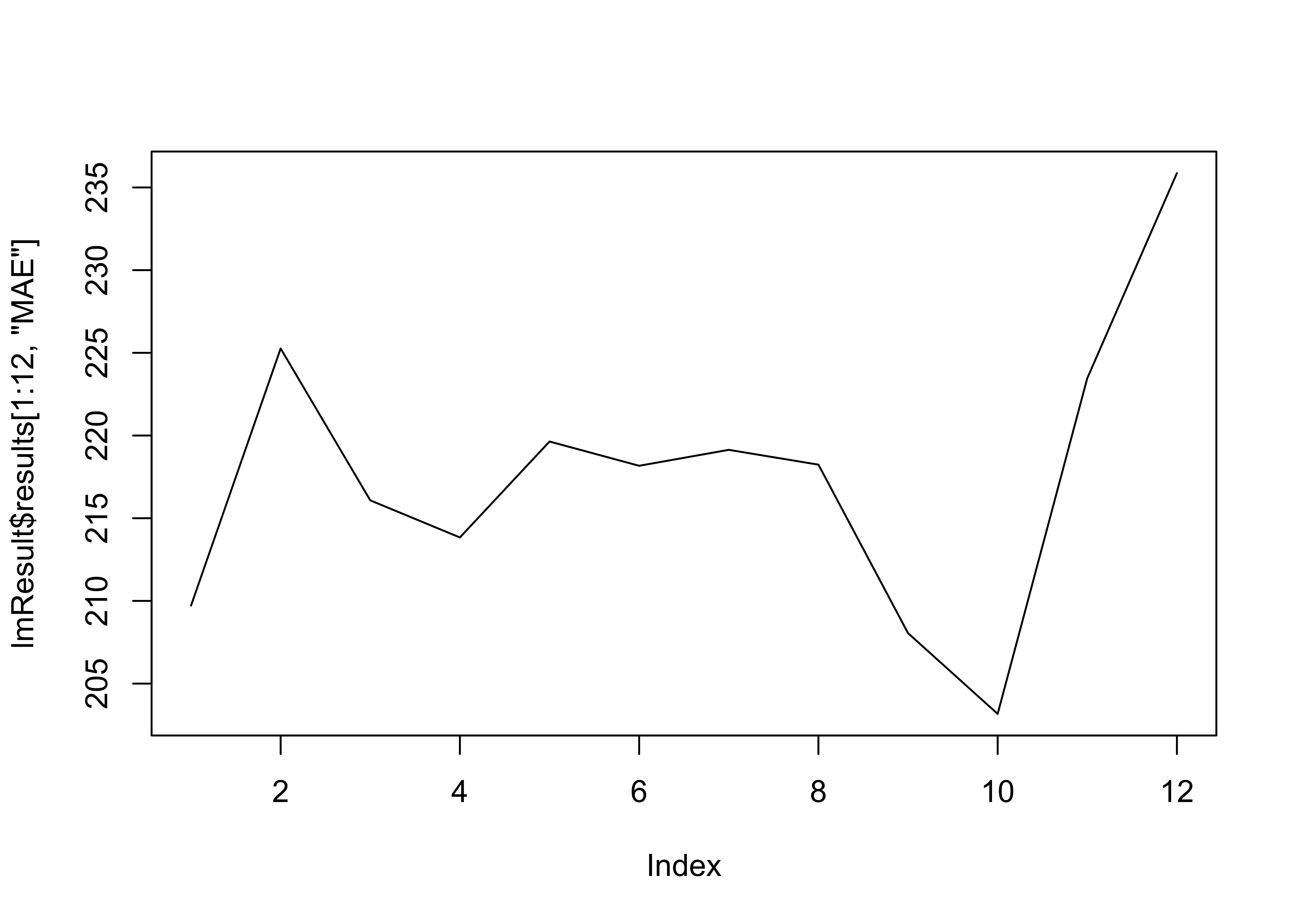
lmResult$results
#>    horizon        ME     RMSE      MAE       MPE      MAPE
#> 1        1 -29.98579 299.6541 209.7159 -3.013060  9.929822
#> 2        2 -29.88039 321.0528 225.2622 -3.194416 10.687050
#> 3        3 -37.60781 309.9057 216.0809 -3.561457 10.471767
#> 4        4 -44.16276 299.9710 213.8367 -3.766603 10.529658
#> 5        5 -46.09350 300.1802 219.6379 -3.733282 11.035018
#> 6        6 -46.71102 305.1078 218.1714 -3.640628 10.997209
#> 7        7 -51.70651 304.0659 219.1350 -3.728902 10.989804
#> 8        8 -53.47684 307.1201 218.2391 -3.624584 10.879932
#> 9        9 -58.65118 298.1247 208.0498 -3.765260 10.306958
#> 10      10 -60.78344 299.8423 203.1693 -3.964980  9.920366
#> 11      11 -60.85124 318.8611 223.4643 -4.173957 10.856528
#> 12      12 -60.73156 341.7946 235.8645 -4.548858 11.437524
#> 13     All -48.38684 308.8067 217.5522 -3.726332 10.670136
arimaResult$results
#>    horizon         ME     RMSE      MAE        MPE     MAPE
#> 1        1  -65.00408 396.7894 311.6545  -6.037641 15.06448
#> 2        2 -139.38596 595.8715 497.5262 -13.509255 26.12166
#> 3        3 -193.32336 706.9039 605.6577 -18.596059 32.68040
#> 4        4 -234.61718 758.8044 667.5272 -21.988430 36.72346
#> 5        5 -259.11651 779.2469 687.7626 -23.943587 38.49269
#> 6        6 -266.47540 768.1292 676.2776 -24.483011 38.37014
#> 7        7 -267.86191 738.4693 650.5500 -24.127737 37.04476
#> 8        8 -264.80720 702.6425 624.6418 -23.351577 35.41462
#> 9        9 -259.03090 660.6630 587.1832 -22.360308 33.25430
#> 10      10 -249.03616 616.2315 546.8732 -21.133686 30.97660
#> 11      11 -246.63815 599.5851 541.2806 -20.945500 30.76113
#> 12      12 -249.43695 621.7274 562.5628 -21.454025 31.80119
#> 13     All -224.56115 662.0887 579.9581 -20.160901 32.22545
plot(lmResult$results[1:12,'MAE'], type='l')
lines(arimaResult$results[1:12,'MAE'], col=2)

I am particularly excited about this code because it will allow me to apply arbitrary machine learning algorithms to forecasting problems. For example, I could create an xreg matrix of lags and use a support vector machine, neural network, or random forest to make 1-step forecasts. I am planning to release this code as a package on CRAN, once I finish the documentation. I’m also planning to re-work the function a bit to return an S3 class, containing:

1. Predicted values at each forecast horizon, including beyond the length of the input time series.
2. Actual values at each forecast horizon, for easy comparison to #1.
3. Matrix of average error at each horizon.
4. The final model.
5. Forecasts using the final model, from the last observation of x to the “max horizon”.
6. A print method that will show #3.
7. A plot method that will plot #3.

Let me know if you have any suggestions or spot any bugs!