Functional and Parallel Time Series Cross-validation

November 21, 2011 • By Zach Deane-Mayer

Rob Hyndman has a great post on his blog with example on how to cross-validate a time series model. The basic concept is simple: You start with a minimum number of observations (k), and fit a model (e.g. an arima model) to those observations. You then forecast out to a certain horizon (h), and compare your forecasts to the actual values for that series. You then add the next observation (k+1), and repeat the process until you run out of data. This gives you a matrix of forecast accuracies at various horizons (1 step ahead, 2 steps ahead, all the way to h steps ahead). You then take the mean of each column of the matrix, and get the model’s average accuracy at that horizon. This method is analogous to leave-one-out cross-validation.

There are 2 variations to this method: 1. Use a fixed training window. In this case, when you add an observation to your “training” series, you drop the first observation, keeping the training window fixed. 2. Increment by n at each step, rather than 1. This is analogous to k-fold cross-validation. In this case, your forecast error is more unstable, and it’s a good idea to average error across ALL horizons when evaluating the model.

This technique is very useful, because it allows you to define a horizon of interest (say 1 month or 12 months), and then asses how well your model performs at that horizon. Furthermore, you can use this data to compare various models, including different types of models, such as linear models vs. arima models vs. exponential smoothing model.

However, time series cross-validation is very time consuming, particularly for arima and exponential smoothing models. Therefore, I thought it would be a good idea to parallelize Hyndman’s algorithm, using the foreach package in R. Furthermore, I wrapped the entire thing into a single function, which allows you to easily change the type of cross validation by altering the minObs (k), stepSize (n), and fixed-length or growing window parameters. My function takes an argument tsControl, which contains each of these parameters, as well a summary function to calculate your error metric (such as MAE). I’ve structured it similarly to the caret packages’s train function.

The FUN argument should be a function that takes 2 parameters: x and h. x is a univariate time series, and h is a forecast horizon. The function should build a model using x, and then return h forecasts. Here are some examples of this function, for linear models, arima models, and exponential smoothing models. As you can see, they all return the same output: a vector of h point forecasts.

devtools::install_github('zachmayer/cv.ts')

Here is my replication of Hyndman’s example. Note that I create a “tsControl” list which contains the parameters for the cross-validation algorithm. This example is not parallelized, but you can easily change that by loading your favorite “foreach” backend, such as doMC or doRedis. Note that parallelization introduces a lot of overhead, and actually seems to slow down the linear model. I recommend only running the more complicated models (such as ets and Arima) in parallel.

set.seed(1)
library(cv.ts)
library(fpp) # To load the data set a10
set.seed(42)

myControl <- tseriesControl(
                  minObs=60,
                  stepSize=1,
                  maxHorizon=12,
                  fixedWindow=FALSE,
                  summaryFunc=tsSummary
                  )
HZ <- 12

#Linear model
LM <- cv.ts(a10, lmForecast, tsControl=myControl, lambda=0, progress=FALSE)

#Arima
AR <- cv.ts(a10, arimaForecast, tsControl=myControl,
        order=c(3,0,1),
        seasonal=list(order=c(0,1,1), period=12),
        include.drift=TRUE,
        lambda=0,
        method="ML",
    progress=FALSE)

#ETS
ETS <- cv.ts(a10, etsForecast, tsControl=myControl, model="MMM", damped=TRUE, progress=FALSE)

#Compare
print(LM$results)
#>    horizon         ME     RMSE       MAE       MPE     MAPE
#> 1        1 -0.2725912 1.076396 0.7791545 -2.614665 5.596926
#> 2        2 -0.2822531 1.082641 0.7871349 -2.710239 5.658250
#> 3        3 -0.2886488 1.092170 0.7976159 -2.770276 5.730474
#> 4        4 -0.2971028 1.104251 0.8103064 -2.852489 5.823448
#> 5        5 -0.3056058 1.109408 0.8189053 -2.931349 5.896185
#> 6        6 -0.3109202 1.118481 0.8248950 -2.954858 5.910637
#> 7        7 -0.3179823 1.127791 0.8343112 -3.013127 5.980584
#> 8        8 -0.3196042 1.130791 0.8345069 -3.005293 5.949104
#> 9        9 -0.3278520 1.140122 0.8434244 -3.049571 5.982685
#> 10      10 -0.3356941 1.149424 0.8525803 -3.082279 6.018591
#> 11      11 -0.3474146 1.157718 0.8618808 -3.177945 6.091796
#> 12      12 -0.3588573 1.165808 0.8711102 -3.257125 6.156913
#> 13     All -0.3137105 1.121250 0.8263188 -2.951601 5.899633
print(AR$results)
#>    horizon          ME      RMSE       MAE       MPE     MAPE
#> 1        1 -0.06952996 0.9576579 0.6864364 -0.987671 5.023620
#> 2        2 -0.08169637 0.9489235 0.6741621 -1.132339 4.872177
#> 3        3 -0.08343977 0.9977603 0.7288596 -1.231540 5.213511
#> 4        4 -0.11067162 1.0439293 0.7385081 -1.559224 5.281564
#> 5        5 -0.10842489 1.0236703 0.7313181 -1.540205 5.253661
#> 6        6 -0.11742386 1.0576470 0.7555417 -1.632494 5.399775
#> 7        7 -0.12813752 1.0642152 0.7660031 -1.733374 5.502634
#> 8        8 -0.12388781 1.0777980 0.7679234 -1.702259 5.483807
#> 9        9 -0.13108887 1.1000320 0.7790721 -1.750583 5.517787
#> 10      10 -0.13214359 1.1176414 0.7948680 -1.748940 5.599111
#> 11      11 -0.13512504 1.1228730 0.8017960 -1.799429 5.660906
#> 12      12 -0.13643063 1.1206344 0.7955103 -1.801673 5.609461
#> 13     All -0.11316666 1.0527318 0.7516666 -1.551644 5.368168
print(ETS$results)
#>    horizon        ME     RMSE       MAE      MPE     MAPE
#> 1        1 0.1132662 1.096961 0.7555067 0.811820 5.341824
#> 2        2 0.1415040 1.074570 0.7507118 1.097761 5.308178
#> 3        3 0.1823720 1.132433 0.8115826 1.338857 5.734240
#> 4        4 0.2481434 1.200547 0.8523130 1.721842 5.982308
#> 5        5 0.2926954 1.139426 0.8375651 2.005419 5.935881
#> 6        6 0.3362320 1.217865 0.8764216 2.336122 6.134923
#> 7        7 0.3962229 1.269369 0.9154994 2.738119 6.414465
#> 8        8 0.4646886 1.305978 0.9461516 3.209884 6.582228
#> 9        9 0.5291823 1.400404 0.9824138 3.658850 6.755941
#> 10      10 0.5935464 1.440317 1.0473199 4.128987 7.180029
#> 11      11 0.6613151 1.453265 1.0377274 4.550946 7.141743
#> 12      12 0.7359366 1.496950 1.0893617 5.081606 7.494982
#> 13     All 0.3912587 1.269007 0.9085479 2.723351 6.333895

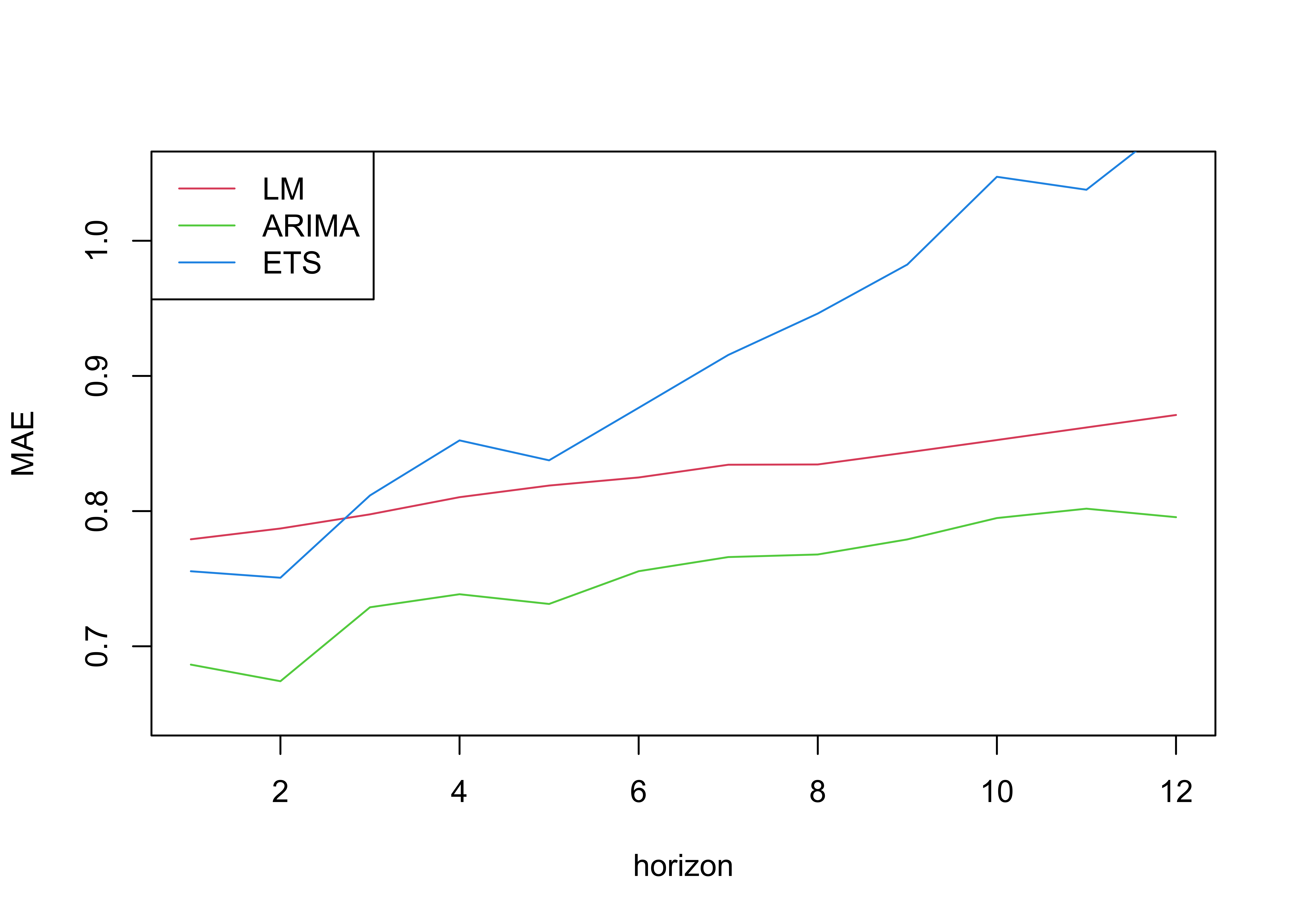
This function produces the same results as Hyndman’s example:

plot(1:12,LM$results[1:HZ,'MAE'], type="l", col=2, xlab="horizon", ylab="MAE",
     ylim=c(0.65,1.05))
lines(1:12, AR$results[1:HZ,'MAE'], type="l",col=3)
lines(1:12, ETS$results[1:HZ,'MAE'], type="l",col=4)
legend("topleft",legend=c("LM","ARIMA","ETS"),col=2:4,lty=1)

A line plot comparing the Mean Absolute Error (MAE) across different forecast horizons for three models: Linear Model (LM), ARIMA, and Exponential Smoothing State Space Model (ETS). The plot shows that the MAE increases for all models as the forecast horizon extends. The ETS model has the highest MAE across most horizons, indicating lower accuracy, while the ARIMA model has the lowest MAE, performing best at shorter horizons. The LM model exhibits a steady increase in MAE with longer horizons, showing moderate performance compared to the other models.

This code is very early stage, and could contain bugs. Please comment if you find one, or if you think of any ways to improve this algorithm. Feel free to try it out with your own forecasting functions!

Functional and Parallel Time Series Cross-validation

stay in touch