Strong Correlation With High P-value

October 21, 2011 • By Zach Deane-Mayer

This post is a repost of a question I asked on Cross Validated back in 2011. The question and its answer were foundational in my understanding of correlation coefficients, so I’m preserving it here.

The Question

I was wondering, is it possible to have a very strong correlation coefficient (say .9 or higher), with a high p value (say .25 or higher)?

Here’s an example of a low correlation coefficient, with a high p value:

set.seed(10)
y <- rnorm(100)
x <- rnorm(100)+.1*y
cor.test(x,y)
#> 
#>  Pearson's product-moment correlation
#> 
#> data:  x and y
#> t = 0.38726, df = 98, p-value = 0.6994
#> alternative hypothesis: true correlation is not equal to 0
#> 95 percent confidence interval:
#>  -0.1585461  0.2337130
#> sample estimates:
#>        cor 
#> 0.03908927

High correlation coefficient, low p value:

y <- rnorm(100)
x <- rnorm(100)+2*y
cor.test(x,y)
#> 
#>  Pearson's product-moment correlation
#> 
#> data:  x and y
#> t = 18.414, df = 98, p-value < 2.2e-16
#> alternative hypothesis: true correlation is not equal to 0
#> 95 percent confidence interval:
#>  0.8275258 0.9183272
#> sample estimates:
#>       cor 
#> 0.8807809

Low correlation coefficient, low p value:

y <- rnorm(100000)
x <- rnorm(100000)+.1*y
cor.test(x,y)
#> 
#>  Pearson's product-moment correlation
#> 
#> data:  x and y
#> t = 32.907, df = 99998, p-value < 2.2e-16
#> alternative hypothesis: true correlation is not equal to 0
#> 95 percent confidence interval:
#>  0.09736627 0.10962941
#> sample estimates:
#>       cor 
#> 0.1035018

High correlation coefficient, high p value: ???

The Answer (by cardinal)

The sample correlation coefficient needed to reject the hypothesis that the true (Pearson) correlation coefficient is zero becomes small quite fast as the sample size increases. So, in general, no, you cannot simultaneously have a large (in magnitude) correlation coefficient and a simultaneously large p-value.

The Details

The test used for the Pearson correlation coefficient in the R function cor.test is a very slightly modified version of the method I discuss below.

Suppose $`(X_1,Y_1),(X_2,Y_2),\ldots,(X_n,Y_n)`$ are iid bivariate normal random vectors with correlation $`\rho`$ . We want to test the null hypothesis that $`\rho=0`$ versus $`\rho\neq 0`$ . Let $`r`$ be the sample correlation coefficient. Using standard linear-regression theory, it is not hard to show that the test statistic,

T=r\frac{\sqrt{n-2}}{\sqrt{(1-r^2)}}

has a $`t_{n-2}`$ distribution under the null hypothesis. For large $`n`$ , the $`t_{n-2}`$ distribution approaches the standard normal. Hence $`T^2`$ is approximately chi-squared distributed with one degree of freedom. (Under the assumptions we’ve made, $`T^2\sim F_{1,n-2}`$ in actuality, but the $`\chi^2_1`$ approximation makes clearer what is going on, I think.)

So,

\mathbb{P}\left(\frac{r^2}{1-r^2}(n-2)\geq q_{1-\alpha}\right)\approx \alpha,

where $`q_{1-\alpha}`$ is the $`(1-\alpha)`$ quantile of a chi-squared distribution with one degree of freedom.

Now, note that $`r^2/(1-r^2)`$ is increasing as $`r^2`$ increases. Rearranging the quantity in the probability statement, we have that for all

|r|\geq\sqrt{\frac{1}{1+(n-2)/q_{1-\alpha}}}

we’ll get a rejection of the null hypothesis at level $`\alpha`$ . Clearly the right-hand side decreases with $`n`$ .

A Plot

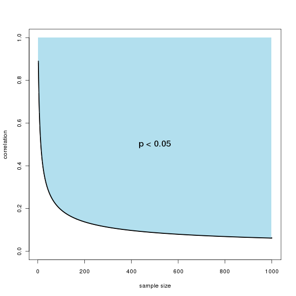
Here is a plot of the rejection region of $`|r|`$ as a function of the sample size. So, for example, when the sample size exceeds 100, the (absolute) correlation need only be about 0.2 to reject the null at the $`\alpha=0.05`$ level.

A Simulation

We can do a simple simulation to generate a pair of zero-mean vectors with an exact correlation coefficient. Below is the code. From this we can look at the output of cor.test.

k <- 100
n <- 4*k

# Correlation that gives an approximate p-value of 0.05
# Change 0.05 to some other desired p-value to get a different curve
pval <- 0.05
qval <- qchisq(pval,1,lower.tail=F)
rho  <- 1/sqrt(1+(n-2)/qval)

# Zero-mean orthogonal basis vectors
b1 <- rep(c(1,-1),n/2)
b2 <- rep(c(1,1,-1,-1),n/4)

# Construct x and y vectors with mean zero and an empirical
# correlation of *exactly* rho
x <- b1
y <- rho * b1 + sqrt(1-rho^2) * b2

# Do test
cor.test(x,y)
#> 
#>  Pearson's product-moment correlation
#> 
#> data:  x and y
#> t = 1.96, df = 398, p-value = 0.0507
#> alternative hypothesis: true correlation is not equal to 0
#> 95 percent confidence interval:
#>  -0.0002810133  0.1939656012
#> sample estimates:
#>       cor 
#> 0.0977734