Kaggle Competition Walkthrough: Wrapup
The Kaggle Don’t Overfit competition is over, and I took 11th place! Additionally, I tied with tks for contributing the most to the forum, so thanks to everyone who voted for me! I voted for tks, and I’m very happy to share the prize with him, as most of my code is based off of his work.
The top finishers in this competition did a writeup of their methods in the forums, and they are definitely worth a read. In my last post, I promised a writeup of a method that would beat the benchmark by a significant margin, so here that is. This variable selection technique is based on tks’ code.
To start, we set things up in the same way as my previous posts: Load the data, split train vs. test, etc. You can find the data for this post here.
#Load Required Packages
library('caTools')
library('caret')
library('glmnet')
library('ipred')
library('e1071')
set.seed(42)

############################
# Load the Data, choose target, create train and test sets
############################

Data <- read.csv("../../../public/data/overfitting.csv", header=TRUE)

#Choose Target
Data$Target <- as.factor(ifelse(Data$Target_Practice ==1,'X1','X0'))
Data$Target_Evaluate = NULL
Data$Target_Leaderboard = NULL
Data$Target_Practice = NULL
xnames <- setdiff(names(Data),c('Target','case_id','train'))

#Order
Data <- Data[,c('Target','case_id','train',xnames)]

#Split to train and test
trainset = Data[Data$train == 1,]
testset = Data[Data$train == 0,]

#Remove unwanted columns
trainset$case_id = NULL
trainset$train = NULL
To improve over our previous attempt, which fits a glmnet model on all 200 variables, we want to select a subset of those variables that performs better than the entire thing. This whole process must be cross-validated to avoid overfitting, but fortunately the caret package in R has a great function called rfe that handles most of the gruntwork. The process is described in great detail here, but it can be thought of as 2 nested loops: the outer loop resamples your dataset, either using cross-validation or bootstrap sampling, and then feeds the resampled data to the inner loop, which fits a model, calculates variable importances based on that model, and then eliminates the least important variables and re-calculates the model’s fit. The results of the inner loop are collected by the outer loop, which then stores a re-sampled metric of each variable’s importance, as well as the number of variables that produced the best fit. If it sounds complicated, read the document at my previous link for more detailed information.
#Custom Functions
glmnetFuncs <- caretFuncs #Default caret functions

glmnetFuncs$summary <-  twoClassSummary

glmnetFuncs$rank <- function (object, x, y) {
    vimp <- sort(object$finalModel$beta[, 1])
    vimp <- as.data.frame(vimp)
    vimp$var <- row.names(vimp)
    vimp$'Overall' <- seq(nrow(vimp),1)
    vimp
}

MyRFEcontrol <- rfeControl(
        functions = glmnetFuncs,
        method = "boot",
        number = 25,
        rerank = FALSE,
        returnResamp = "final",
        saveDetails = FALSE,
        verbose = FALSE)
This section of code initializes an object to control the RFE function. We use the ‘caretFuncs’ object as our framework, and the ‘twoClassSummary’ function as our summary function, as we are doing a 2-class problem and want to use AUC to evaluate our predictive accuracy. Then we use a custom function to rank the variables from a fitted glmnet object, based on tks’ method. We’ve decided to rank the variables by their coefficients, and consider variables with larger coefficients more important. I’m still not 100% sure why this worked for this competition, but it definitely gives better results than glmnet on its own. Finally, we create our RFE control object, where we specify that we want to use 25 repeats of bootstrap sampling for our outer loop.
Next, we have to setup the training parameters and multicore parameters, all of which are explained in my previous posts. In both loops of my RFE function I am using 25 repeats of bootstrap sampling, which you could turn up to 50 or 100 for higher accuracy at the cost of longer runtimes.
####################################
# Training parameters
####################################
MyTrainControl=trainControl(
        method = "boot",
        number=25,
        returnResamp = "all",
        classProbs = TRUE,
        summaryFunction=twoClassSummary
        )

####################################
# Setup Multicore
####################################
#source:
#http://www.r-bloggers.com/feature-selection-using-the-caret-package/
if ( require("multicore", quietly = TRUE, warn.conflicts = FALSE) ) {
    MyRFEcontrol$workers <- multicore:::detectCores()
    MyRFEcontrol$computeFunction <- mclapply
    MyRFEcontrol$computeArgs <- list(mc.preschedule = FALSE, mc.set.seed = FALSE)

    MyTrainControl$workers <- multicore:::detectCores()
    MyTrainControl$computeFunction <- mclapply
    MyTrainControl$computeArgs <- list(mc.preschedule = FALSE, mc.set.seed = FALSE)
}
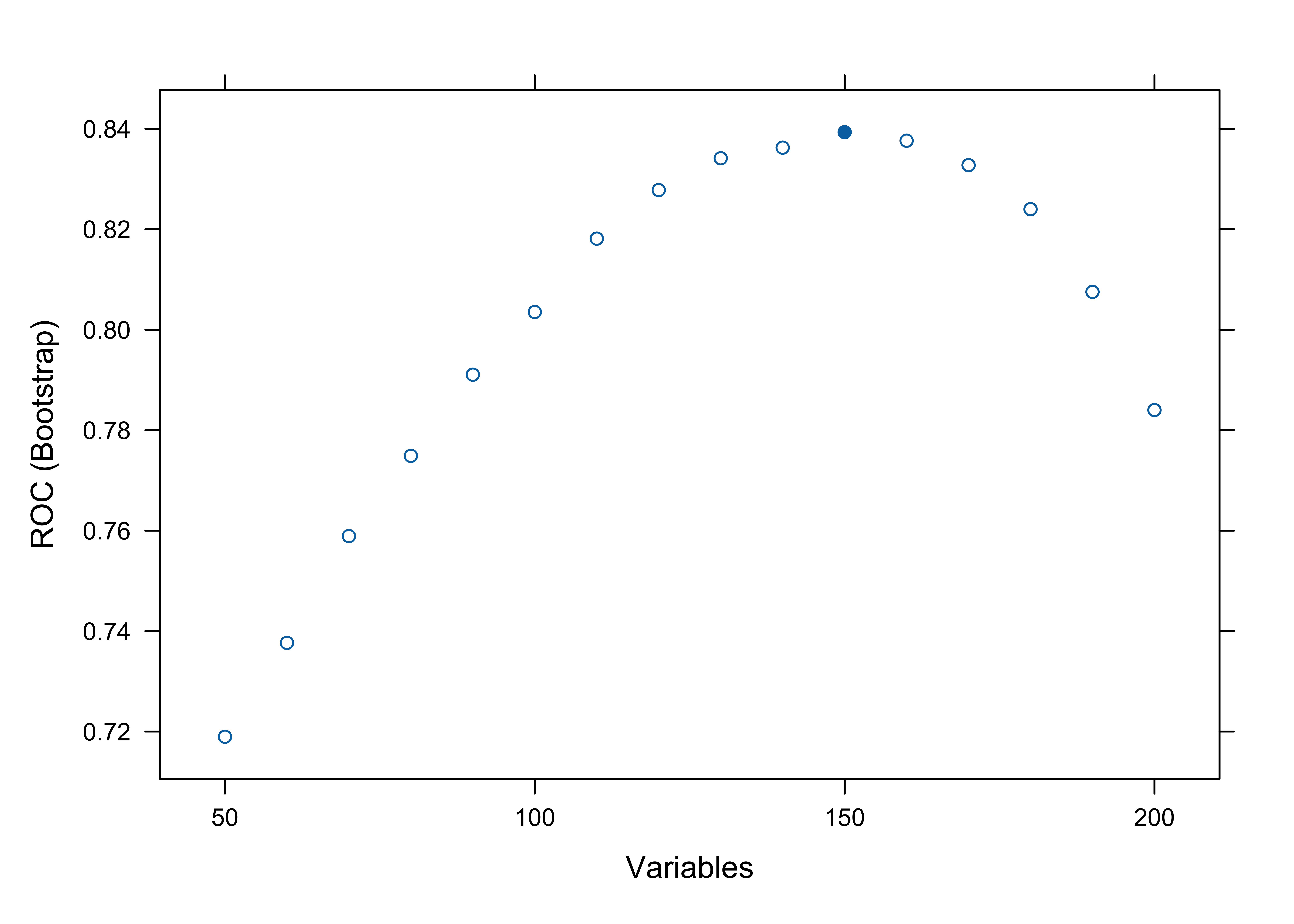
Now we get to actually run the RFE function and recursively eliminate features! The structure of the RFE function is very similar to caret’s train function. In fact, the inner loop of RFE is fitting a model using the train function, so we need to pass 2 sets of parameters to RFE: one for RFE and one for train. I have indented the parameters for the train function twice so you can see what’s going on. After running RFE, we can access the variables it selected using RFE$optVariables, which we use to construct a formula we will use to fit the final model. We can also plot the RFE object for a graphical representation of how well the various subsets of variables performed.
####################################
# Select Features-GLMNET
####################################

x <- trainset[,xnames]
y <- trainset$Target

RFE <- rfe(x,y,sizes = seq(50,200,by=10),
        metric = "ROC",maximize=TRUE,rfeControl = MyRFEcontrol,
            method='glmnet',
            tuneGrid = expand.grid(.alpha=0,.lambda=c(0.01,0.02)),
            trControl = MyTrainControl)

NewVars <- RFE$optVariables
RFE
#>
#> Recursive feature selection
#>
#> Outer resampling method: Bootstrapped (25 reps)
#>
#> Resampling performance over subset size:
#>
#>  Variables    ROC   Sens   Spec   ROCSD  SensSD  SpecSD Selected
#>         50 0.7190 0.6432 0.6783 0.05210 0.08389 0.08094
#>         60 0.7377 0.6723 0.6687 0.06024 0.08639 0.09233
#>         70 0.7589 0.6835 0.6940 0.04983 0.06826 0.07608
#>         80 0.7749 0.7046 0.6986 0.04771 0.07136 0.07112
#>         90 0.7910 0.7055 0.7058 0.04292 0.07473 0.07565
#>        100 0.8035 0.7116 0.7283 0.04077 0.06758 0.07341
#>        110 0.8181 0.7350 0.7398 0.04001 0.06274 0.07041
#>        120 0.8278 0.7361 0.7559 0.03982 0.07787 0.05128
#>        130 0.8341 0.7465 0.7571 0.04500 0.08234 0.04886
#>        140 0.8362 0.7613 0.7569 0.04458 0.08980 0.04709
#>        150 0.8393 0.7577 0.7611 0.04534 0.08705 0.05480        *
#>        160 0.8376 0.7531 0.7601 0.04629 0.09329 0.05267
#>        170 0.8328 0.7549 0.7507 0.04323 0.08861 0.05354
#>        180 0.8240 0.7506 0.7448 0.03941 0.07698 0.05576
#>        190 0.8075 0.7317 0.7267 0.04258 0.08836 0.05963
#>        200 0.7840 0.7092 0.7024 0.04496 0.07977 0.05879
#>
#> The top 5 variables (out of 150):
#>    var_127, var_40, var_50, var_117, var_47
plot(RFE)

FL <- as.formula(paste("Target ~ ", paste(NewVars, collapse= "+"))) #RFE
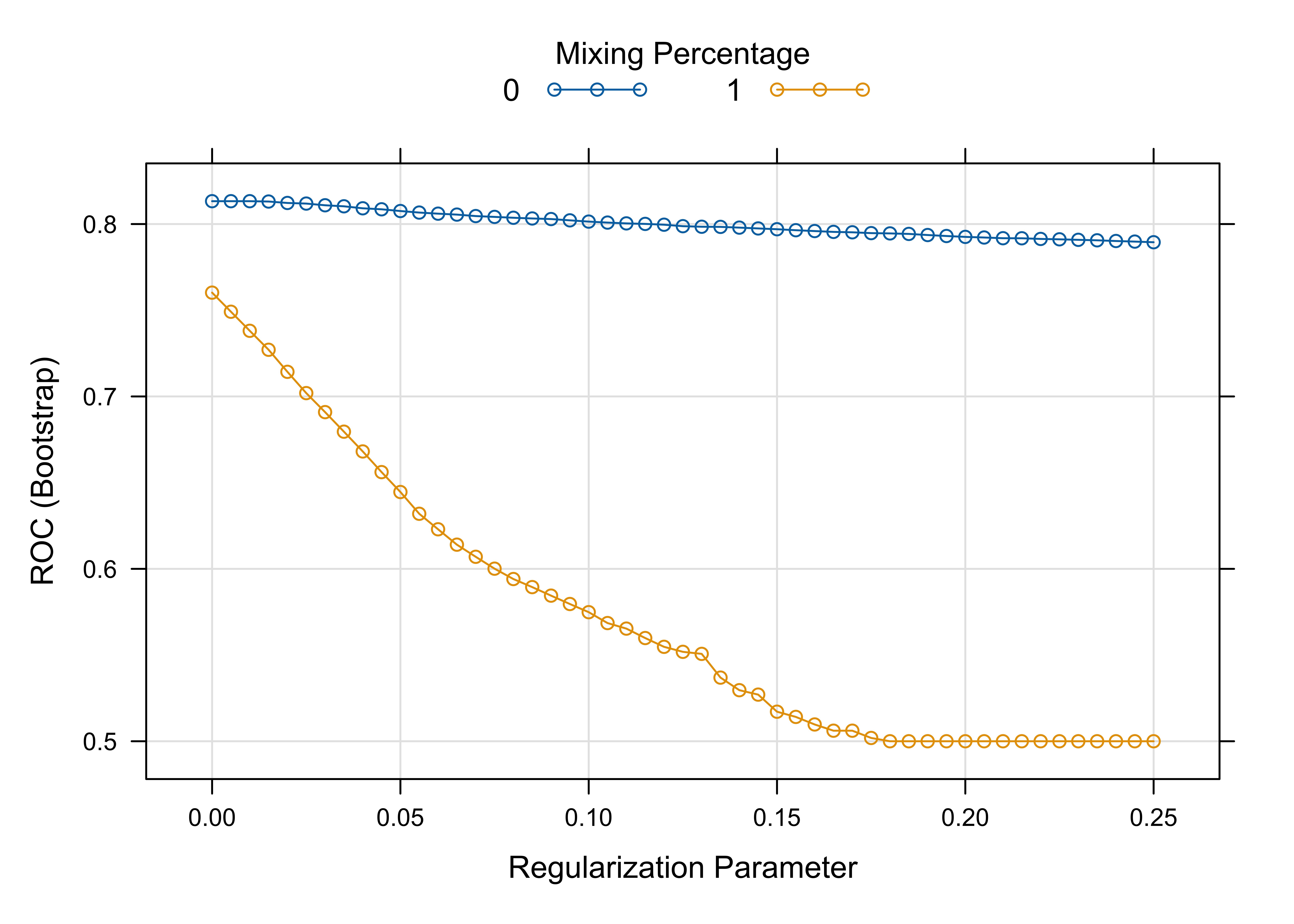
Lastly, we fit our final model using caret’s train function. This step is a little unnecessary, because RFE also fit a final model on the full dataset, but I included it anyways to try out a longer sequence of lambdas (lambda is a parameter for the glmnet model).
####################################
# Fit a GLMNET Model
####################################

model <- train(FL,data=trainset,method='glmnet',
    metric = "ROC",
    tuneGrid = expand.grid(.alpha=c(0,1),.lambda=seq(0,.25,by=0.005)),
    trControl=MyTrainControl)
model
#> glmnet
#>
#> 250 samples
#> 150 predictors
#>   2 classes: 'X0', 'X1'
#>
#> No pre-processing
#> Resampling: Bootstrapped (25 reps)
#> Summary of sample sizes: 250, 250, 250, 250, 250, 250, ...
#> Resampling results across tuning parameters:
#>
#>   alpha  lambda  ROC        Sens        Spec
#>   0      0.000   0.8132591  0.68980719  0.7522959
#>   0      0.005   0.8132591  0.68980719  0.7522959
#>   0      0.010   0.8132591  0.68980719  0.7522959
#>   0      0.015   0.8130658  0.68980719  0.7531848
#>   0      0.020   0.8122312  0.69136578  0.7515381
#>   0      0.025   0.8118779  0.68782421  0.7497540
#>   0      0.030   0.8108937  0.68516793  0.7507101
#>   0      0.035   0.8102945  0.68395338  0.7480973
#>   0      0.040   0.8091388  0.68066412  0.7481058
#>   0      0.045   0.8085559  0.68163973  0.7489119
#>   0      0.050   0.8075556  0.67988128  0.7488956
#>   0      0.055   0.8066630  0.67904954  0.7483028
#>   0      0.060   0.8060282  0.67813863  0.7516721
#>   0      0.065   0.8054803  0.67562018  0.7508581
#>   0      0.070   0.8046305  0.67396630  0.7499800
#>   0      0.075   0.8041495  0.67299069  0.7507963
#>   0      0.080   0.8036523  0.67201508  0.7510393
#>   0      0.085   0.8032376  0.66954487  0.7502230
#>   0      0.090   0.8028997  0.66503045  0.7504380
#>   0      0.095   0.8021493  0.66397567  0.7518703
#>   0      0.100   0.8014228  0.66149637  0.7527213
#>   0      0.105   0.8008523  0.65965120  0.7529322
#>   0      0.110   0.8003858  0.65880013  0.7544308
#>   0      0.115   0.8000858  0.65886688  0.7527087
#>   0      0.120   0.7996223  0.65793665  0.7527976
#>   0      0.125   0.7987628  0.65761874  0.7528865
#>   0      0.130   0.7984421  0.65761874  0.7530113
#>   0      0.135   0.7983576  0.65749419  0.7531360
#>   0      0.140   0.7979343  0.65749419  0.7563085
#>   0      0.145   0.7974560  0.65571290  0.7571973
#>   0      0.150   0.7969976  0.65571290  0.7572699
#>   0      0.155   0.7964269  0.65480381  0.7564699
#>   0      0.160   0.7959351  0.65480381  0.7564699
#>   0      0.165   0.7954501  0.65480381  0.7564699
#>   0      0.170   0.7952161  0.65227954  0.7565763
#>   0      0.175   0.7947402  0.65235674  0.7557599
#>   0      0.180   0.7945706  0.65148717  0.7573776
#>   0      0.185   0.7942806  0.65148717  0.7573776
#>   0      0.190   0.7936313  0.65235674  0.7581776
#>   0      0.195   0.7930642  0.65144765  0.7581776
#>   0      0.200   0.7925503  0.65057808  0.7565044
#>   0      0.205   0.7921994  0.64885745  0.7565044
#>   0      0.210   0.7917880  0.64885745  0.7589044
#>   0      0.215   0.7917501  0.64885745  0.7588866
#>   0      0.220   0.7913681  0.64798789  0.7571009
#>   0      0.225   0.7911450  0.64514271  0.7571009
#>   0      0.230   0.7908512  0.64514271  0.7571009
#>   0      0.235   0.7905719  0.64514271  0.7571009
#>   0      0.240   0.7901655  0.64333276  0.7571009
#>   0      0.245   0.7898248  0.64233276  0.7562314
#>   0      0.250   0.7894533  0.64146319  0.7562314
#>   1      0.000   0.7602176  0.63852965  0.7174748
#>   1      0.005   0.7491402  0.62134660  0.7182409
#>   1      0.010   0.7380795  0.61901816  0.7096195
#>   1      0.015   0.7270782  0.60554500  0.7058009
#>   1      0.020   0.7142875  0.59527048  0.6965156
#>   1      0.025   0.7019364  0.58655556  0.6947302
#>   1      0.030   0.6909100  0.57376807  0.6858545
#>   1      0.035   0.6795716  0.56751437  0.6766293
#>   1      0.040   0.6681012  0.55544937  0.6717075
#>   1      0.045   0.6561183  0.54409354  0.6746432
#>   1      0.050   0.6445707  0.53662606  0.6670787
#>   1      0.055   0.6319519  0.52463805  0.6628462
#>   1      0.060   0.6229534  0.51049653  0.6662347
#>   1      0.065   0.6140283  0.49563846  0.6647388
#>   1      0.070   0.6069947  0.47678933  0.6737063
#>   1      0.075   0.6001067  0.45086355  0.6731632
#>   1      0.080   0.5940988  0.43249009  0.6842088
#>   1      0.085   0.5894126  0.41443712  0.6900603
#>   1      0.090   0.5844673  0.39913393  0.6934504
#>   1      0.095   0.5796093  0.38006212  0.7095700
#>   1      0.100   0.5748729  0.35263941  0.7311311
#>   1      0.105   0.5685571  0.31936808  0.7445395
#>   1      0.110   0.5653412  0.29250544  0.7672510
#>   1      0.115   0.5598690  0.24678963  0.8025435
#>   1      0.120   0.5547730  0.21151657  0.8231986
#>   1      0.125   0.5518743  0.18838182  0.8455542
#>   1      0.130   0.5506827  0.16458268  0.8681920
#>   1      0.135   0.5369172  0.14224229  0.8840181
#>   1      0.140   0.5296231  0.13928953  0.8759836
#>   1      0.145   0.5270547  0.14935874  0.8635804
#>   1      0.150   0.5171469  0.14111130  0.8691612
#>   1      0.155   0.5141192  0.13556721  0.8745385
#>   1      0.160   0.5097371  0.11158827  0.8968840
#>   1      0.165   0.5061286  0.09743590  0.9050847
#>   1      0.170   0.5061286  0.09538462  0.9091525
#>   1      0.175   0.5019122  0.08102564  0.9200000
#>   1      0.180   0.5000000  0.08000000  0.9200000
#>   1      0.185   0.5000000  0.08000000  0.9200000
#>   1      0.190   0.5000000  0.08000000  0.9200000
#>   1      0.195   0.5000000  0.08000000  0.9200000
#>   1      0.200   0.5000000  0.08000000  0.9200000
#>   1      0.205   0.5000000  0.08000000  0.9200000
#>   1      0.210   0.5000000  0.08000000  0.9200000
#>   1      0.215   0.5000000  0.08000000  0.9200000
#>   1      0.220   0.5000000  0.08000000  0.9200000
#>   1      0.225   0.5000000  0.08000000  0.9200000
#>   1      0.230   0.5000000  0.08000000  0.9200000
#>   1      0.235   0.5000000  0.08000000  0.9200000
#>   1      0.240   0.5000000  0.08000000  0.9200000
#>   1      0.245   0.5000000  0.08000000  0.9200000
#>   1      0.250   0.5000000  0.08000000  0.9200000
#>
#> ROC was used to select the optimal model using the largest value.
#> The final values used for the model were alpha = 0 and lambda = 0.01.
plot(model, metric='ROC')

test <- predict(model, newdata=testset, type  = "prob")
colAUC(test, testset$Target)
#>                  X0        X1
#> X0 vs. X1 0.9012783 0.9012783

predictions <- test

########################################
#Generate a file for submission
########################################
testID  <- testset$case_id
submit_file = data.frame('Zach'=predictions[,1])
# write.csv(submit_file, file="AUC_ZACH.txt", row.names = FALSE)
Because we fit our model on Target_Practice, we can score the model ourselves using colAUC. This model gets .91 on Target_Practice, and also scored about .91 on Target_Leaderboard and Target_Evaluate. Unfortunately, .91 was only good for 80th place on the leaderboard, asOckham released the set of variables used for the leaderboard dataset, and I was unable to fit a good model using this information. Many other competitors were able to use this information to their advantage, but this yielded no edge on the final Target_Evaluate, which is what really mattered.
Overall, I’m very happy with the result of this competition. If anyone has any code they’d like to share that scored higher than .96 on the leaderboard, I’d be happy to hear from you!