Kaggle Competition Walkthrough: Fitting a Model
Now that we’ve got the data we need into R, it is very easy to fit a model using the caret package. Caret’s workhorse function is called ‘train,’ and it allows you to fit a wide variety of models using the same syntax. Furthermore, many models have ‘hyperparameters’ that require tuning, such as the number of neighbors for a KNN model or the regularization parameters for an elastic net model. Caret tunes these parameters using a ‘grid’ search, and will either define a reasonable grid for you, or allow you to specify one yourself. For example, you might want to investigate KNN models with 3,5, and 10 neighbors. ‘Train’ will use cross-validation or bootstrap re-sampling to evaluate the predictive performance of each model, and then will fit the final model on your complete training dataset.
You can find the data for this post here.
set.seed(42)
Data <- read.csv("../../../public/data/overfitting.csv", header=TRUE)

#Choose Target
Data$Target <- as.factor(ifelse(Data$Target_Practice ==1,'X1','X0'))
Data$Target_Evaluate = NULL
Data$Target_Leaderboard = NULL
Data$Target_Practice = NULL
xnames <- setdiff(names(Data),c('Target','case_id','train'))

#Order
Data <- Data[,c('Target','case_id','train',xnames)]

#Split to train and test
trainset = Data[Data$train == 1,]
testset = Data[Data$train == 0,]

#Remove unwanted columns
trainset$case_id = NULL
trainset$train = NULL

FL <- as.formula(paste("Target ~ ", paste(xnames, collapse= "+")))
First, we define some parameters to pass to caret’s ‘train’ function:
library(caret)
MyTrainControl=trainControl(
        method = "repeatedCV",
        number=10,
        repeats=5,
        returnResamp = "all",
        classProbs = TRUE,
        summaryFunction=twoClassSummary
        )
We use the ‘trainControl’ function to define train parameters. In this case, we want to use a repeated cross-validation re-sampling strategy, so we will employ a 10-fold cross-validation and repeat it 5 times. Furthermore, we want train to return class probabilities, because this competition is scored using the AUC metric, which requires probabilities. Finally, we use the twoClassSummary function, which calculates useful metrics for evaluating the predictive performance of a 2-class classification model. This final line is very important, as it will allow cart to evaluate our model using AUC.
Next, we fit our model:
model <- train(FL,data=trainset,method='glmnet',
    metric = "ROC",
    tuneGrid = expand.grid(.alpha=c(0,1),.lambda=seq(0,0.05,by=0.01)),
    trControl=MyTrainControl)
print(model)
#> glmnet
#>
#> 250 samples
#> 200 predictors
#>   2 classes: 'X0', 'X1'
#>
#> No pre-processing
#> Resampling: Cross-Validated (10 fold, repeated 5 times)
#> Summary of sample sizes: 226, 225, 225, 225, 225, 225, ...
#> Resampling results across tuning parameters:
#>
#>   alpha  lambda  ROC        Sens       Spec
#>   0      0.00    0.8495313  0.7618182  0.7743956
#>   0      0.01    0.8495313  0.7618182  0.7743956
#>   0      0.02    0.8467125  0.7601515  0.7760440
#>   0      0.03    0.8445621  0.7566667  0.7774725
#>   0      0.04    0.8436430  0.7433333  0.7790110
#>   0      0.05    0.8424958  0.7416667  0.7759341
#>   1      0.00    0.8046978  0.7330303  0.7297802
#>   1      0.01    0.7817358  0.7015152  0.7158242
#>   1      0.02    0.7605611  0.6590909  0.7021978
#>   1      0.03    0.7313636  0.6216667  0.7004396
#>   1      0.04    0.6953330  0.5642424  0.6916484
#>   1      0.05    0.6681285  0.5507576  0.6760440
#>
#> ROC was used to select the optimal model using the largest value.
#> The final values used for the model were alpha = 0 and lambda = 0.01.
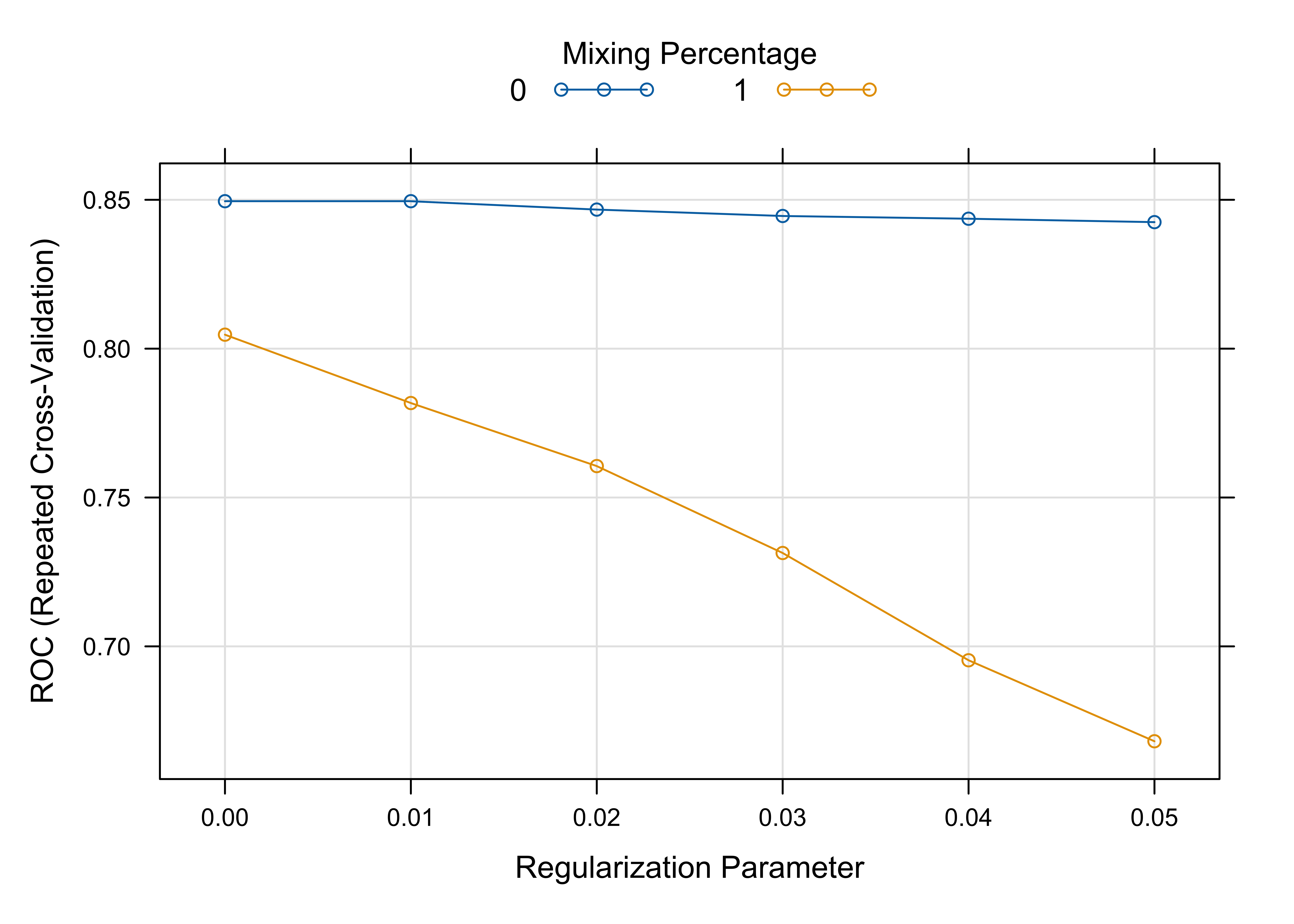
plot(model, metric='ROC')

You may recall in my last post, I defined a formula called ‘FL,’ which we are now using to specify our model. You could also specify the model using x,y form, where x is a matrix of independent variables and y is your dependent variables. This second method is a little bit faster, but I find using the formula interface makes my code easier to read and modify, which is FAR more important. Next we specify that we want to fit the model to the training set, and that we want to use the ‘glmnet’ model. Glmnet uses the elastic net, and performs quiet well on this dataset. Also, the Kaggle benchmark uses glmnet, so it is a good place to start. Next, we specify the metric, ROC (which really means AUC), by which the candidate models will be ranked. Then, we specify a custom tuning grid, which I found produces some nice results. You could also instead specify tuneLength=5 here to allow train to build its own grid, but in this case I prefer some finer control over the hyperparameters that get passed to ‘train.’ Finally, we pass the control object we defined earlier to the train function, and we’re off!
After fitting the model, it is useful to look at how various glmnet hyperparameters affected its performance. Additionally, we can score on our test set, because we chose to use ‘Target_Practice’ as our target, and this Target has a known evaluate set.
library(caTools)
test <- predict(model, newdata=testset, type  = "prob")
colAUC(test, testset$Target)
#>                  X0        X1
#> X0 vs. X1 0.8678578 0.8678578
We get an AUC of 0.8682391, which is pretty much equivalent to the benchmark of .87355. In my next post, I will show you how to beat the benchmark (and the majority of the other competitors) by a significant margin.
Update: Furthermore, if you are on a linux machine, and wish to speed this process up, run the following code snippet after you define the parameters for your training function: This will replace ‘lapply’ with ‘mclapply’ in caret’s train function, and will allow you simultaneously fit as many models as your machine has cores. Isn’t technology great? Also note that this code will not run in the Mac Gui. You need to open up the terminal and start R by typing ‘R’ to run your script in the console. The Mac gui does not handle ‘multicore’ well…
#source: http://www.r-bloggers.com/feature-selection-using-the-caret-package/
if ( require("multicore", quietly = TRUE, warn.conflicts = FALSE) ) {
    MyTrainControl$workers <- multicore:::detectCores()
    MyTrainControl$computeFunction <- mclapply
    MyTrainControl$computeArgs <- list(mc.preschedule = FALSE, mc.set.seed = FALSE)
}