Error Metrics for Multi-class Problems in R: Beyond Accuracy and Kappa

July 6, 2012 • By Zach Deane-Mayer

The caret package for R provides a variety of error metrics for regression models and 2-class classification models, but only calculates Accuracy and Kappa for multi-class models. Therefore, I wrote the following function to allow caret::train to calculate a wide variety of error metrics for multi-class problems:

#Multi-Class Summary Function
#Based on caret::twoClassSummary
require(compiler)
require(pROC)
multiClassSummary <- cmpfun(function (data, lev = NULL, model = NULL){

  #Load Libraries
  require(Metrics)
  require(caret)

  #Check data
  if (!all(levels(data[, "pred"]) == levels(data[, "obs"])))
    stop("levels of observed and predicted data do not match")

  #Calculate custom one-vs-all stats for each class
  prob_stats <- lapply(levels(data[, "pred"]), function(class){

    #Grab one-vs-all data for the class
    pred <- ifelse(data[, "pred"] == class, 1, 0)
    obs  <- ifelse(data[,  "obs"] == class, 1, 0)
    prob <- data[,class]

    #Calculate one-vs-all AUC and logLoss and return
    cap_prob <- pmin(pmax(prob, .000001), .999999)
    prob_stats <- c(auc(obs, prob), logLoss(obs, cap_prob))
    names(prob_stats) <- c('ROC', 'logLoss')
    return(prob_stats)
  })
  prob_stats <- do.call(rbind, prob_stats)
  rownames(prob_stats) <- paste('Class:', levels(data[, "pred"]))

  #Calculate confusion matrix-based statistics
  CM <- confusionMatrix(data[, "pred"], data[, "obs"])

  #Aggregate and average class-wise stats
  #Todo: add weights
  class_stats <- cbind(CM$byClass, prob_stats)
  class_stats <- colMeans(class_stats)

  #Aggregate overall stats
  overall_stats <- c(CM$overall)

  #Combine overall with class-wise stats and remove some stats we don't want
  stats <- c(overall_stats, class_stats)
  stats <- stats[! names(stats) %in% c('AccuracyNull',
    'Prevalence', 'Detection Prevalence')]

  #Clean names and return
  names(stats) <- gsub('[[:blank:]]+', '_', names(stats))
  return(stats)

})

This function was prompted by a question on cross-validated, asking what the optimal value of k is for a knn model fit to the iris dataset. I wanted to look at statistics besides accuracy and kappa, so I wrote a wrapper function for caret::confusionMatrix and auc and logLoss from the Metric packages. Use the following code to fit a knn model to the iris dataset:

library(caret)
set.seed(19556)
model <- train(
  Species~.,
  data=iris,
  method='knn',
  tuneGrid=expand.grid(.k=1:30),
  metric='Accuracy',
  trControl=trainControl(
    method='repeatedcv',
    number=10,
    repeats=15,
    classProbs=TRUE,
    summaryFunction=multiClassSummary))

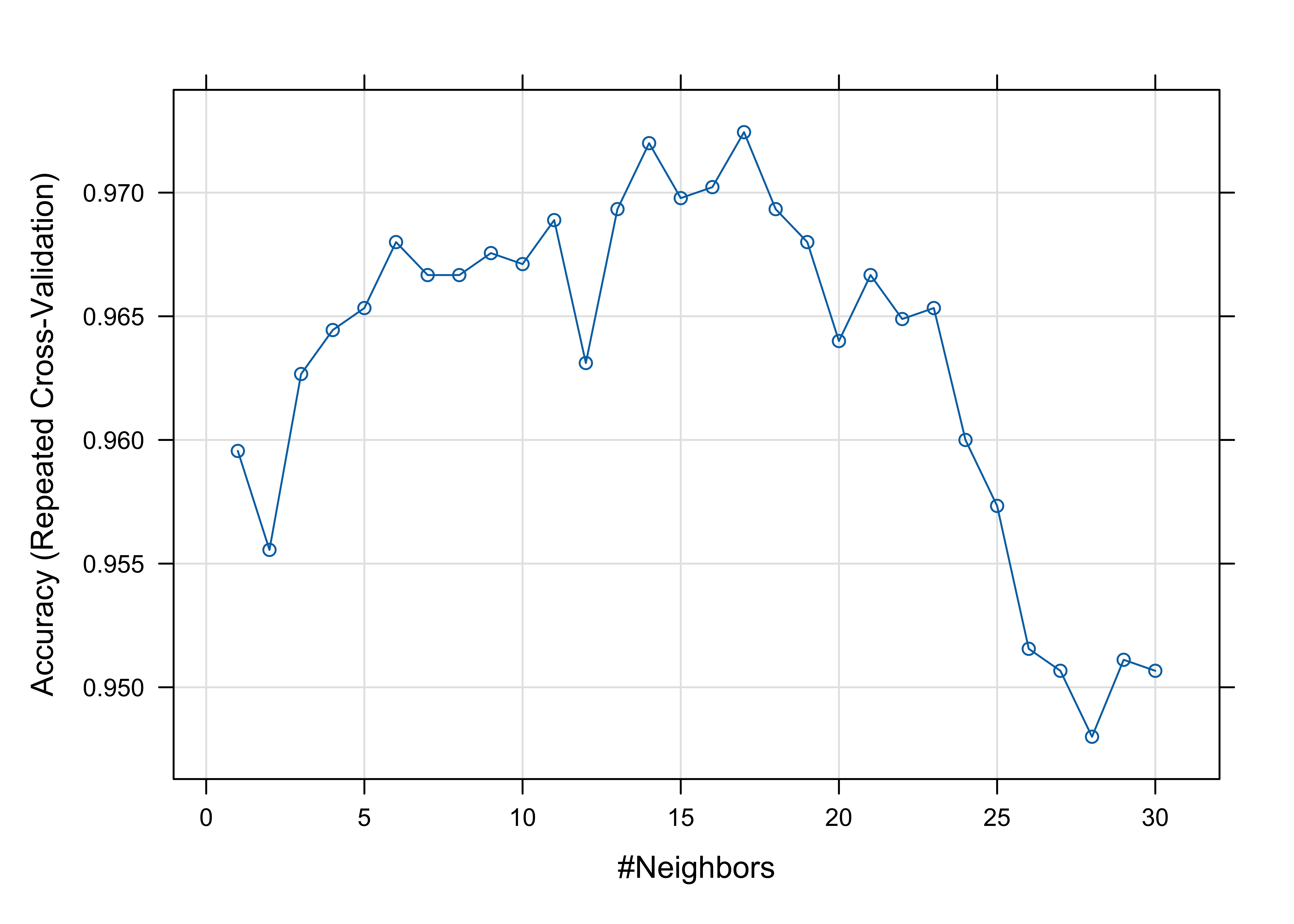
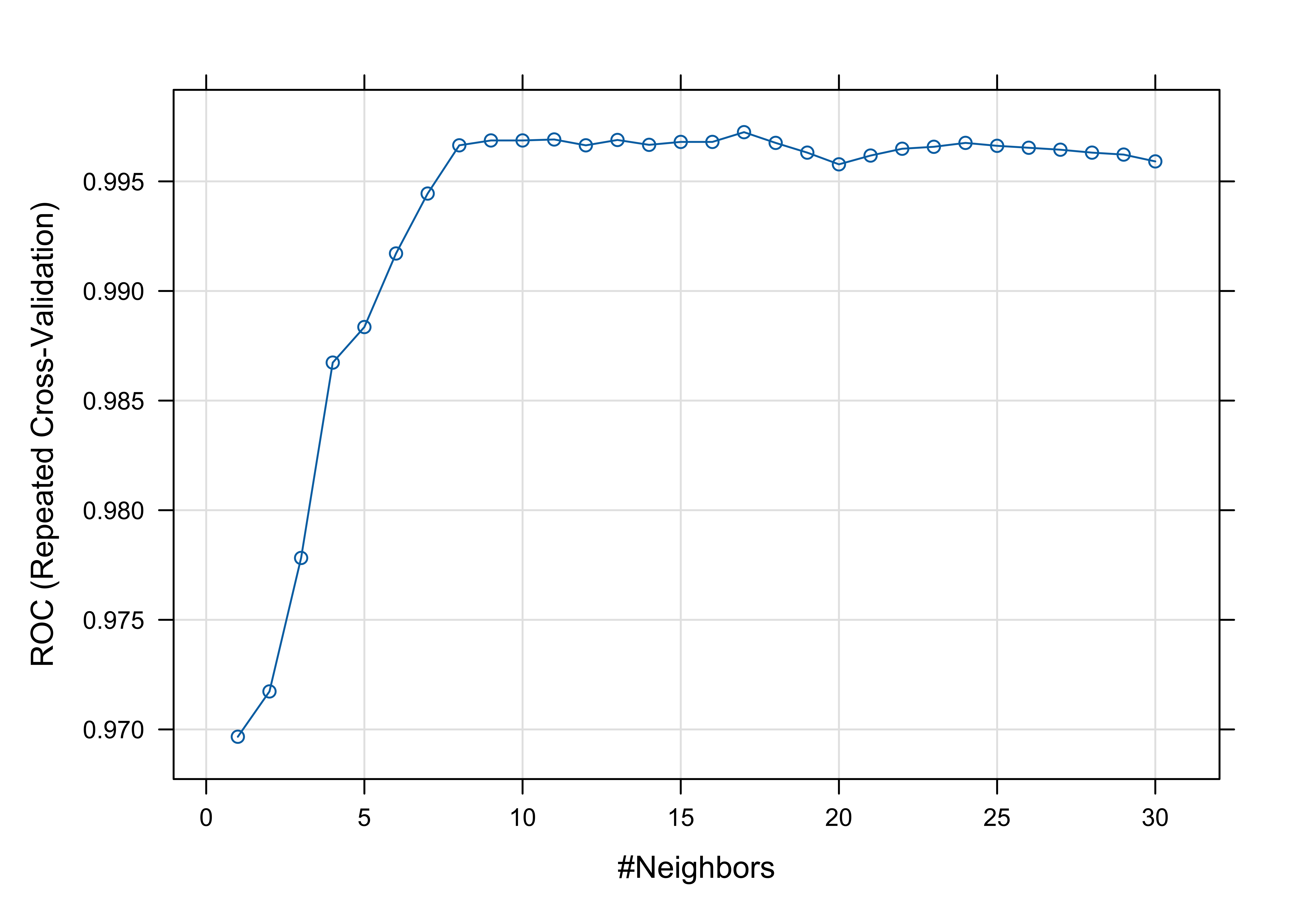
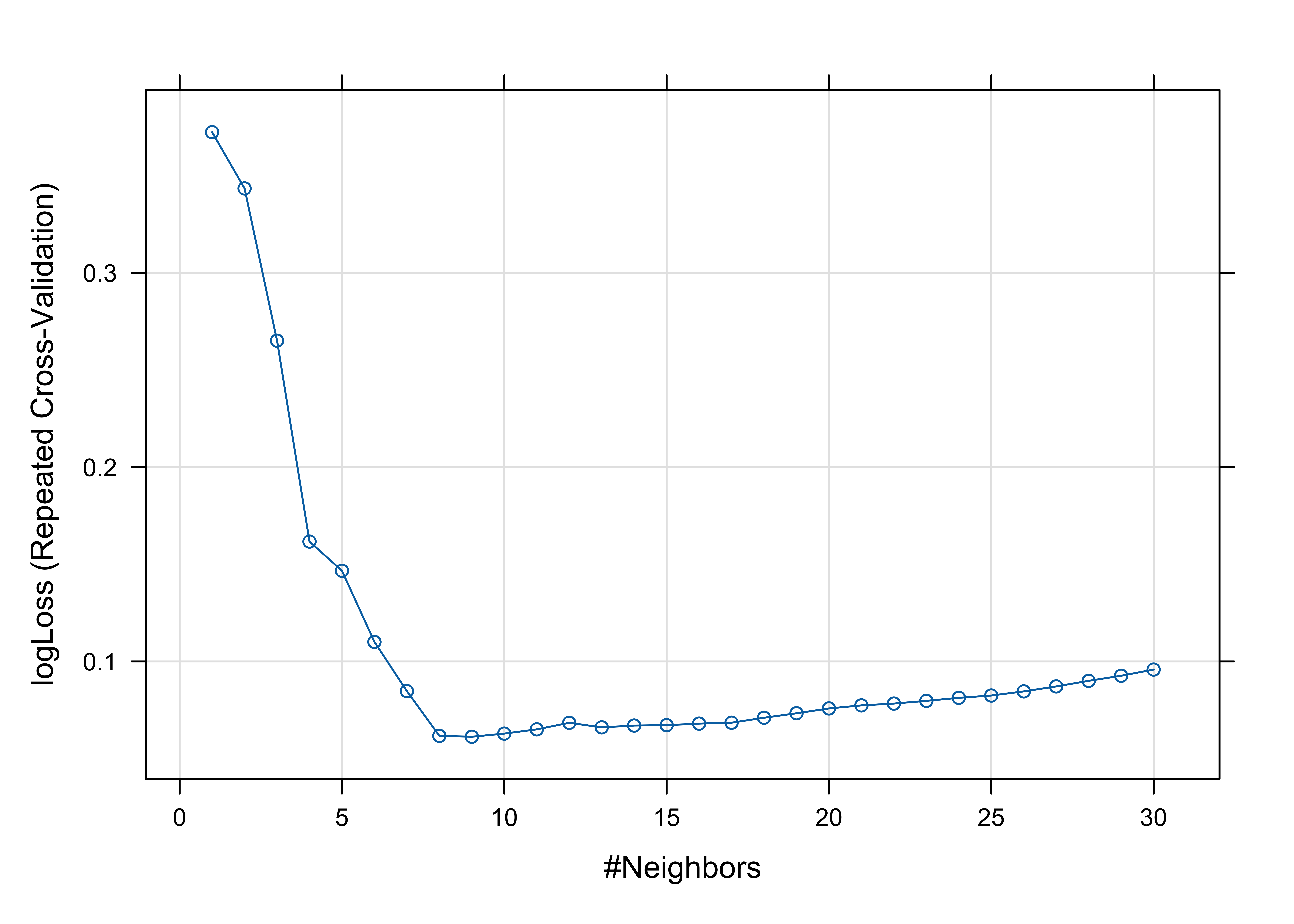
This demonstrates that, depending on what metric you use, you will end up with a different model. For example, Accuracy seems to peak around 17, while AUC and logLoss seem to peak around 6:

# All possible metrics:
# c('Accuracy', 'Kappa', 'AccuracyLower', 'AccuracyUpper', 'AccuracyPValue',
#               'Sensitivity', 'Specificity', 'Pos_Pred_Value',
#               'Neg_Pred_Value', 'Detection_Rate', 'ROC', 'logLoss')
print(plot(model, metric='Accuracy'))

A line plot showing the relationship between the number of neighbors in a k-nearest neighbors (k-NN) algorithm and the model's accuracy, measured through repeated cross-validation. The plot indicates that accuracy increases as the number of neighbors increases, peaking around 15 neighbors, after which accuracy declines as the number of neighbors continues to increase.

print(plot(model, metric='ROC'))

A line plot showing the relationship between the number of neighbors in a k-nearest neighbors (k-NN) algorithm and the ROC AUC, measured through repeated cross-validation. The plot shows that the ROC AUC increases rapidly with the number of neighbors, reaching a plateau around 10 neighbors, and then remains relatively stable, indicating strong model performance for neighbor counts between 10 and 30.

print(plot(model, metric='logLoss'))

A line plot depicting the relationship between the number of neighbors in a k-nearest neighbors (k-NN) algorithm and the log loss, measured through repeated cross-validation. The plot shows that log loss decreases sharply as the number of neighbors increases from 0 to 10, reaching a minimum around 10 neighbors, after which log loss gradually increases as the number of neighbors continues to increase.

You can also increase the number of cross-validation repeats, or use a different method of re-sampling, such as bootstrap re-sampling.

Error Metrics for Multi-class Problems in R: Beyond Accuracy and Kappa

stay in touch