Don't Overfit II - My First Place Solution

This was my solution write-up for the Don’t Overfit II competition. It originally appeared on Kaggle, but I’m reposting it here as well.

First place solution

First of all, I want to say that I feel incredibly honored to win. The original Don’t Overfit was my first Kaggle competition and coincides with when I discovered machine learning. I remember poring over forum posts to learn how to fit models with the caret package and writing R code on the commuter train on my way to job interviews in Boston, a city where I’d just arrived. On those train rides, I daydreamed about one day having a job where I did machine learning for work.

I can’t believe it’s been 8 years.

The original Don’t Overfit competition was the start of a trajectory that took me to the career I have today. Thank you @salimali for piquing my interest, and thank you to the Kaggle community for all you’ve given to me.

This competition, of course, was completely different from the original Don’t Overfit 😁

In the original competition, we only had 5 submissions total for the private leaderboard and no leaderboard feedback.

I believe my critical insight was being among the first to realize leaderboard probing would be key to winning. I started a dedicated effort to submit every individual variable as a single submission. I was able to get the AUC for all 300 variables on the public leaderboard, and as @cdeotte already discussed, used (AUC public) - 0.50 to come up with “coefficients” based on AUC. If Chris had had time for 250 more submissions, he would have had a good chance of beating me. Just using the 300 public LB “coefficients”, with no further processing, gives a private LB score of 0.853, which would have been good enough for 110th place or so.

I additionally used the AUCs on the training data to add a little bit of extra information to this model, using the following formula: 0.11*(AUC train) + 0.89*(AUC pubic) - 0.5 The weight for AUC train is (rows train)/[rows train + rows public] The weight for AUC public is (rows public)/[rows train + rows public]

This gives a private leaderboard score of 0.856, good enough for 60th place or so. (About where I finished in the first iteration of Don’t Overfit!).

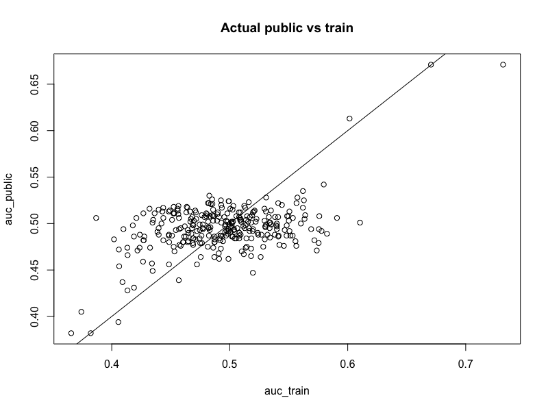
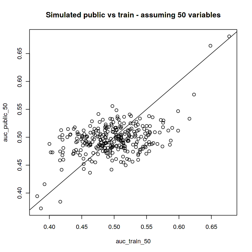
It also gives the following plot of public AUC vs training AUC, which led me to believe all 300 variables were used to create the target variable. This is also a useful plot to calibrate simulated datasets (more on this later):

This methodology overfits the public leaderboard, as there are many small AUCs that should probably be zero. Using Chris’ capping heuristic, we can set every coefficient with abs(cf) < 0.04 = 0, which yields the following equation:

-0.0661*X16 + -0.0448*X29 + 0.1778*X33 + -0.0526*X45 + -0.0736*X63 + 0.171*X65 + -0.059*X70 + -0.1047*X73 + -0.118*X91 + -0.0422*X106 + -0.0446*X108 + -0.0985*X117 + -0.0448*X132 + 0.0462*X164 + -0.0514*X189 + 0.1117*X199 + -0.0704*X209 + -0.1198*X217 + -0.0456*X239

This is very similar to Chris’ solution, just with more variables. This gives a private leaderboard score of 0.877, which is good enough for first place.

I don’t like capping, and I wanted a solution that smoothly shrinks smaller AUCs to zero. For example, variable 239 in the above equation has a coefficient of -0.0456, and there’s a good chance that is really a zero (but I’m not certain)!

So what I spent most of my time doing was looking for an equation that would smoothly shrink small coefficients to zero, while leaving large coefficients more or less alone. I dove down a bit of a rabbit hole here, but it was a fun rabbit hole, and I’m interested to see what approaches other people take to solving the same problem.

The approach I took was:

1. Simulate a dataset with 20,000 rows, 300 columns, sampled from the random normal distribution. AKA matrix(rnorm(20000*300), ncol=300) in R. I am 99.99% sure this is how Kaggle simulated the data for this competition.
2. Apply my probed coefficients to the data. This isn’t perfect, but the coefficients I probed should be pretty representative of the real distribution of coefficients. AKA matrix(rnorm(20000*300), ncol=300) %*% probed_cf in R.
3. Add a little random noise.
4. Choose a classification cutoff that gives a target distribution in the training data of 160 0s and 90 1s.

I then fiddled with steps 2-4 until I got (AUC train - 250 rows) vs (AUC public - 1975 rows) plots that looked like the above plot.

I also simulated “leaderboard probing” to try to get simulated results that had training AUCs of .95 and public AUCs around .92, as those were my results on the real leaderboard.

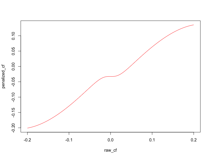
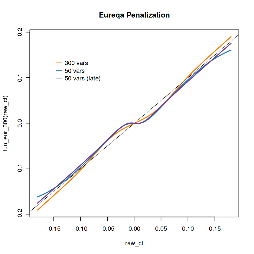
Once I had my simulated data, the problem becomes: predict the “real” coefficients, given the probed coefficients. I played around with many different methodologies for this, and finally ended up using Eureqa Desktop to discover the following equation:

penalized_cf = 0.0320794465661013 + 1.38501844798023*cf - 9.51464300036321*cf^3 - 
    0.0654557703259389*plogis(85.9772069321308*cf)

(Where plogis is the sigmoid function in R)

Here is a plot of the penalized coefficients vs. the raw coefficients. Note that coefficients near zero get shrunk almost completely to zero, but not entirely:

So to recap, my final submission was:

cf = 0.11*(auc_train) + 0.89*(auc_pubic) - 0.5
penalized_cf = 0.032 + 1.385*cf - 9.515*cf^3 - 0.065*plogis(85.977*cf)
sub = X_sub %*% penalized_cf

This achieves a private LB score of 0.886 and a public LB score of 0.923

I’ll post more detailed code (along with the probed AUCs) in some public kernels.

---

Comments:

As a follow up, here are the 300 probed AUCs as a kernel and as a dataset: https://www.kaggle.com/zachmayer/300-probed-aucs?scriptVersionId=13927278 https://www.kaggle.com/zachmayer/300-probed-aucs-from-dont-overfit-ii

And here’s my code: https://www.kaggle.com/zachmayer/first-place-solution?scriptVersionId=13934694

Full code

This is the complete code implementation of my solution. You can also view it on Kaggle.

Load the probed public LB AUCs

library(data.table)
public_aucs_csv <- fread("../input/300-probed-aucs-from-dont-overfit-ii/probed_aucs.csv")
public_aucs <- public_aucs_csv[['public_auc']]
names(public_aucs) <- public_aucs_csv[['variable']]

Load the competition data

# Read the data
dat_train <- fread('../input/dont-overfit-ii/train.csv')
dat_test <- fread("../input/dont-overfit-ii/test.csv")

# Clean the data a bit
dat_train[,id := NULL]
setnames(dat_train, make.names(names(dat_train)))
setnames(dat_test, make.names(names(dat_test)))

# Split into X matrices and a y vector
X_train <- as.matrix(dat_train[,setdiff(names(dat_train), c('id', 'target')),with=F])
X_sub <- as.matrix(dat_test[,colnames(X_train),with=F])
y_train <- dat_train[,target]

Calculate training AUCs

# Fast AUC function
# https://stat.ethz.ch/pipermail/r-help/2005-September/079872.html
fastAUC <- function (x, y){
  x1 = x[y == 1]
  x2 = x[y == 0]
  n1 = as.numeric(length(x1))
  n2 = as.numeric(length(x2))
  r = rank(c(x1, x2))
  auc = (sum(r[1:n1]) - n1 * (n1 + 1)/2)/(n1 * n2)
  return(auc)
}

fastcolAUC <- function(X, y){
  apply(X, 2, function(x) fastAUC(x, y))
}

train_aucs = fastcolAUC(X_train, y_train)
public_aucs = public_aucs[names(train_aucs)]  # Sort the 2 vectors of AUCs in the same order
plot(public_aucs ~ train_aucs)
abline(a=0, b=1)
title("Actual public vs train")

Combine training/public AUCs into coefficients

train_rows <- 250
test_rows <- 19750
public_split <- .10
public_rows <- test_rows * public_split
private_rows <- test_rows * (1-public_split)

total_rows = train_rows + public_rows
train_weight = (train_rows/total_rows)
public_weight = (public_rows/total_rows)
combined_aucs = train_weight*train_aucs + public_weight*public_aucs
coefficients = combined_aucs - .5

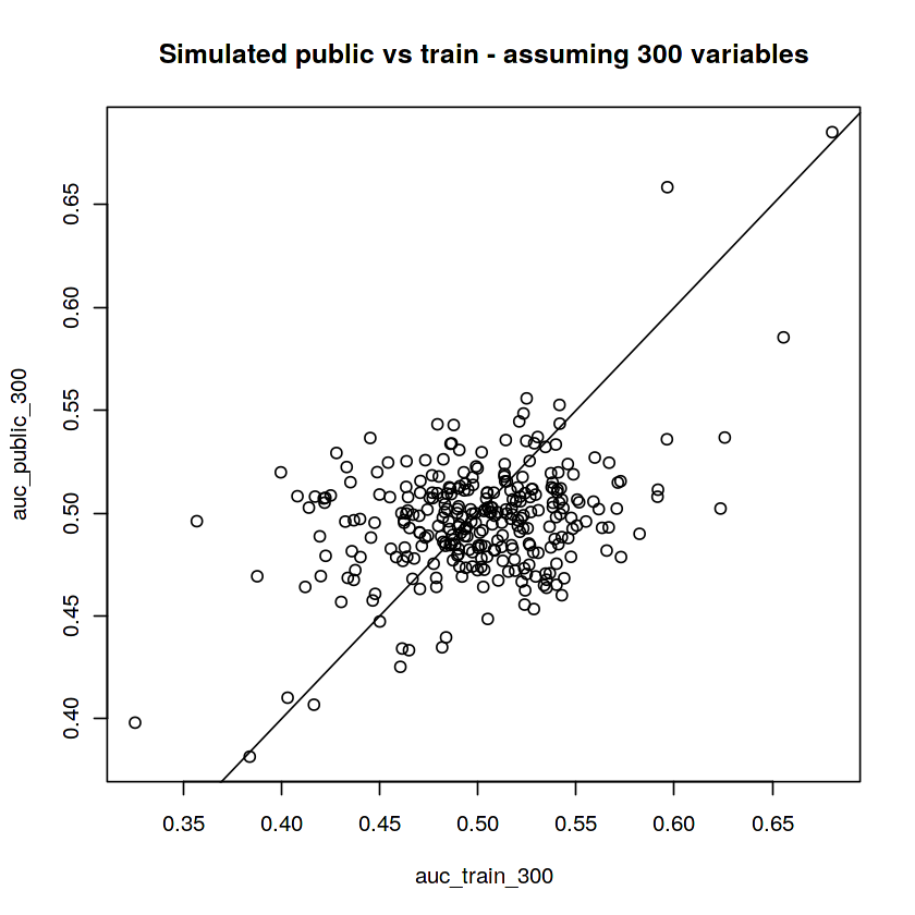
Simulate a dataset with 300 variables

I was convinced this was the true nature of the problem— all 300 vars were used in the target

# Simulate training data
set.seed(1234)
ncols <- 300
X_train <- matrix(rnorm(ncols * train_rows), ncol = ncols)
X_public <- matrix(rnorm(ncols * public_rows), ncol = ncols)
X_private <- matrix(rnorm(ncols * private_rows), ncol = ncols)

# Apply known coefficients to the simulated data and add noise
coefficients_300 <- coefficients
y_train <- (X_train %*% coefficients_300)[,1] + runif(nrow(X_train))/1.5 
y_public <- (X_public %*% coefficients_300)[,1] + runif(nrow(X_public))/1.5
y_private <- (X_private %*% coefficients_300)[,1] + runif(nrow(X_private))/1.5

# Cut the y variable into 0 vs 1
CUT <- sort(y_train)[90]
y_train <- as.integer(y_train > CUT)
y_public <- as.integer(y_public > CUT)
y_private <- as.integer(y_private > CUT)

# Calculate AUCs.  This simulates the competition: auc_train is the training data, auc_public is leaderboard probing, auc_private is unknown
auc_train_300 <- fastcolAUC(X_train, y_train)
auc_public_300 <- fastcolAUC(X_public, y_public)
auc_private_300 <- fastcolAUC(X_private, y_private)

# Plot AUCs.  They should look similar to the first plot in this kernel
plot(auc_public_300 ~ auc_train_300)
abline(a=0, b=1)
title("Simulated public vs train - assuming 300 variables")

# Look at how the AUCs "score" on the public data.  Tweak the simulation until these match what you see on the public LB:
auc_train_pub_priv <- function(x){
  x <- x - 0.5
  pred_train <- X_train %*% x
  pred_public <- X_public %*% x
  pred_private <- X_private %*% x
  out <- c(
    fastAUC(pred_train, y_train),
    fastAUC(pred_public, y_public), 
    fastAUC(pred_private, y_private)
  )
  round(out, 3) 
}
# Model 1: mean of all the training variables
auc_train_pub_priv(rep(1, 300))  # real life is (0.395, 0.433, ?????) (train, pub, priv)
# Output: 0.508 0.445 0.43

# Model 2: AUCs based on training data only
auc_train_pub_priv(auc_train_300)    # real life is c(0.984, 0.739, ?????) (train, pub, priv)
# Output: 0.978 0.699 0.722

# Model 3: AUCs based on public LB probing
auc_train_pub_priv(auc_public_300)   # real life is c(0.907, 0.926, ?????) (train, pub, priv)  - AUCs based only on the public LB data
# Output: 0.828 0.953 0.882

Simulate a dataset with 50 variables

This was my “backup solution” and ended up doing slightly better on the private LB. I was expecting the real solution to have 300 variables, but it looks like 50 was more on the mark.

coefficients_50 <- coefficients[order(abs(coefficients))]
coefficients_50[1:250] <- 0

# Apply known coefficients to the simulated data and add noise
y_train <- (X_train %*% coefficients)[,1] + runif(nrow(X_train))/1.5 
y_public <- (X_public %*% coefficients)[,1] + runif(nrow(X_public))/1.5
y_private <- (X_private %*% coefficients)[,1] + runif(nrow(X_private))/1.5

# Cut the y variable into 0 vs 1
CUT <- sort(y_train)[90]
y_train <- as.integer(y_train > CUT)
y_public <- as.integer(y_public > CUT)
y_private <- as.integer(y_private > CUT)

# Calculate AUCs.  This simulates the competition: auc_train is the training data, auc_public is leaderboard probing, auc_private is unknown
auc_train_50 <- fastcolAUC(X_train, y_train)
auc_public_50 <- fastcolAUC(X_public, y_public)
auc_private_50 <- fastcolAUC(X_private, y_private)

# Plot AUCs.  They should look similar to the first plot in this kernel
plot(auc_public_50 ~ auc_train_50)
abline(a=0, b=1)
title("Simulated public vs train - assuming 50 variables")

# Model 1: mean of all the training variables
auc_train_pub_priv(rep(1, 300))  # real life is (0.395, 0.433, ?????) (train, pub, priv)
# Output: 0.469 0.433 0.422

# Model 2: AUCs based on training data only
auc_train_pub_priv(auc_train_50)    # real life is c(0.984, 0.739, ?????) (train, pub, priv)
# Output: 0.974 0.744 0.73

# Model 3: AUCs based on public LB probing
auc_train_pub_priv(auc_public_50)   # real life is c(0.907, 0.926, ?????) (train, pub, priv)  - AUCs based only on the public LB data
# Output: 0.881 0.951 0.884

Use Eureqa to map train/public AUCs back to original coefficients

Now that we’ve made some simulated datasets, let’s save them to csvs, and see if we can recover the original coefficients, given the public AUCs

# Weight the simulated AUCs the same as we did for the real data
auc_combined_300 = train_weight*auc_train_300 + public_weight*auc_public_300
auc_combined_50 = train_weight*auc_train_50 + public_weight*auc_public_50

# Subtract 0.5 to convert the AUCs to coefficients
cf_combined_300 = auc_combined_300 - .5
cf_combined_50 = auc_combined_50 - .5

# I decided I wanted "symmetrical" equations, so I also saved the inverse of the AUC/CF pairs

# Save the Eureqa training data for 300 variables
out_1 <- data.table(
    probed_cf=auc_combined_300 - .5,
    real_cf=coefficients_300
)
out_2 <- data.table(
    probed_cf=auc_combined_300 - .5,
    real_cf=coefficients_300
)
out <- rbind(out_1, out_2)
head(out)
fwrite(out, 'auc_training_300.csv')

# Save the Eureqa training data for 50 variables
out_1 <- data.table(
    probed_cf=auc_combined_50 - .5,
    real_cf=coefficients_50
)
out_2 <- data.table(
    probed_cf=auc_combined_50 - .5,
    real_cf=coefficients_50
)
out <- rbind(out_1, out_2)
head(out)
fwrite(out, 'auc_training_50.csv')

# Fit eureqa models on auc_training_300.csv using MAE and auc_training_50.csv using MSE
# Sample data:
# probed_cf  real_cf
# 0.02141135    0.0067727840
# -0.02425625   -0.0176978777
# 0.01337607    0.0087553059
# 0.01539266    0.0002067728
# 0.01049981    0.0065633583
# 0.03411041    0.0074291511
# probed_cf real_cf
# 0.03156445    0
# -0.03582437   0
# 0.01420129    0
# 0.02499649    0
# 0.01321816    0
# 0.03663362    0

Now fire up Eureqa desktop and run some searches

I turned on sigmoid functions in my searches - I used MAE for the 300 variable search - I used MSE for the 50 variable search

# These were my 2 real submissions:

# 1. 300 vars (I was so sure of this!)
fun_eur_300 <- function(cf){
    1.05780402210757*cf*plogis(0.0750590053462814 + 339.425848223982*cf^2) - 0.000308402162785152
}

# 2. 50 vars (backup plan)
fun_eur_50 <- function(cf){
    0.0320794465661013 + 1.38501844798023*cf - 9.51464300036321*cf^3 - 0.0654557703259389*plogis(85.9772069321308*cf)
}

# Not submitted
# I ran Eureqa again while writing up this submission and got a simpler 50 variable equation that yields the same result on the public/private LB
fun_eur_50_take_2 <- function(cf){
    cf + cf/(-0.885812581588299 - 1189.09418473067*cf^2)
}

raw_cf <- seq(-.18, .18, length=1000)
plot(fun_eur_300(raw_cf)~raw_cf, col='#ff7f00', type='l', lwd = 2)
lines(fun_eur_50(raw_cf)~raw_cf, col='#1f78b4', type='l', lwd = 2)
lines(fun_eur_50_take_2(raw_cf)~raw_cf, col='#6a3d9a', type='l', lwd = 2)
abline(a=0, b=1, lty='dotted')
legend(-.15, .15, legend=c("300 vars", "50 vars", "50 vars (late)"), col=c("#ff7f00", "#1f78b4", "#6a3d9a"), lty=1, bty = "n")
title("Eureqa Penalization")

Now make submissions based on the eureqa equations

# Model 1: 300 vars - 0.930 public / .880 private
sub_300 <- data.frame(
  'id' = dat_test[['id']], 
  'target' = (X_sub %*% fun_eur_300(coefficients))[,1]
)
fwrite(sub_300, 'sub_300.csv')

# Model 2: 50 vars - 0.923 public / 0.886 private
sub_50 <- data.frame(
  'id' = dat_test[['id']], 
  'target' = (X_sub %*% fun_eur_50(coefficients))[,1]
)
fwrite(sub_50, 'sub_50.csv')

# Model 3: 50 vars (post deadline) - 0.923 public / 0.886 private
sub_50 <- data.frame(
  'id' = dat_test[['id']], 
  'target' = (X_sub %*% fun_eur_50_take_2(coefficients))[,1]
)
fwrite(sub_50, 'sub_50_post_deadline.csv')