caretEnsemble 4.0

August 20, 2024 • By Zach Deane-Mayer

caretEnsemble is a package for creating stacked ensembles of models in R. I’ve been working on this package for over a decade, and I’m proud that it’s still useful even after all these years!

I first wrote this package when I was active on Kaggle, as model stacks are a common technique for winning Kaggle competitions. I loved using the caret package to cross-validate models in R, and caretEnsemble was born out of all my custom R scripts for stacking caret models. I wrote the first draft of caretEnsemble when I was on an Amtrak train from New York to Boston in 2013, and I’ve been maintaining it ever since.

caretEnsemble 4.0, the first update in years, introduces several new features. The highlight is the reintroduction of the greedy ensembling algorithm. This algorithm, present in version 0.0 but removed from the 1.0 CRAN submission due to complexity, has been reimplemented in a clean, modular way. I’m proud of the new implementation: it will be much more maintainable in the future.

This greedy selection algorithm was first described in Ensemble Selection from Libraries of Models and it has some nice properties: 1. The weights of the component models are always positive (negative weights can lead to odd results on out-of-sample data). 2. If it is hard to find a good ensemble, the greedy optimizer will simply select the best single model.

At the end of the day, it’s a simple weighted average of the input models, which turns out to be a robust way to combine models. But if you like complexity, you can also use caretEnsemble to do more complex stacks, using any caret model for the ensemble model. Many winning Kaggle solutions used XGboost to ensemble a variety of input models.

Version 4.0 adds a lot of new features, including greedy stacks, multiclass support, support for mixed-type ensembles, and transfer learning.

Greedy Ensemble demo

First, you will likely need to install the package from CRAN:

install.packages("caretEnsemble", repos = "https://cloud.r-project.org/")

For this demo, I’m going to use the “AmesHousing” and the ranger package, so you should install those too.

install.packages(c("AmesHousing", "Xgboost"), repos = "https://cloud.r-project.org/")

Take a quick look at the data:

set.seed(42)
dat <- AmesHousing::make_ames()
head(dat)
#> # A tibble: 6 × 81
#>   MS_SubClass        MS_Zoning Lot_Frontage Lot_Area Street Alley Lot_Shape Land_Contour Utilities Lot_Config Land_Slope
#>   <fct>              <fct>            <dbl>    <int> <fct>  <fct> <fct>     <fct>        <fct>     <fct>      <fct>
#> 1 One_Story_1946_an… Resident…          141    31770 Pave   No_A… Slightly… Lvl          AllPub    Corner     Gtl
#> 2 One_Story_1946_an… Resident…           80    11622 Pave   No_A… Regular   Lvl          AllPub    Inside     Gtl
#> 3 One_Story_1946_an… Resident…           81    14267 Pave   No_A… Slightly… Lvl          AllPub    Corner     Gtl
#> 4 One_Story_1946_an… Resident…           93    11160 Pave   No_A… Regular   Lvl          AllPub    Corner     Gtl
#> 5 Two_Story_1946_an… Resident…           74    13830 Pave   No_A… Slightly… Lvl          AllPub    Inside     Gtl
#> 6 Two_Story_1946_an… Resident…           78     9978 Pave   No_A… Slightly… Lvl          AllPub    Inside     Gtl
#> # ℹ 70 more variables: Neighborhood <fct>, Condition_1 <fct>, Condition_2 <fct>, Bldg_Type <fct>, House_Style <fct>,
#> #   Overall_Qual <fct>, Overall_Cond <fct>, Year_Built <int>, Year_Remod_Add <int>, Roof_Style <fct>, Roof_Matl <fct>,
#> #   Exterior_1st <fct>, Exterior_2nd <fct>, Mas_Vnr_Type <fct>, Mas_Vnr_Area <dbl>, Exter_Qual <fct>, Exter_Cond <fct>,
#> #   Foundation <fct>, Bsmt_Qual <fct>, Bsmt_Cond <fct>, Bsmt_Exposure <fct>, BsmtFin_Type_1 <fct>, BsmtFin_SF_1 <dbl>,
#> #   BsmtFin_Type_2 <fct>, BsmtFin_SF_2 <dbl>, Bsmt_Unf_SF <dbl>, Total_Bsmt_SF <dbl>, Heating <fct>, Heating_QC <fct>,
#> #   Central_Air <fct>, Electrical <fct>, First_Flr_SF <int>, Second_Flr_SF <int>, Low_Qual_Fin_SF <int>,
#> #   Gr_Liv_Area <int>, Bsmt_Full_Bath <dbl>, Bsmt_Half_Bath <dbl>, Full_Bath <int>, Half_Bath <int>, …

To make things a little easier for this demo, we’ll model the log of the sale price, and also center and scale it:

dat$Sale_Price <- log(dat$Sale_Price)
dat$Sale_Price <- scale(dat$Sale_Price, center=TRUE, scale=TRUE)

Now let’s split it into a training set and a test set:

set.seed(780L)
train_index <- caret::createDataPartition(dat$Sale_Price, p = 0.8, list = FALSE)
train_data <- dat[train_index, ]
test_data <- dat[-train_index, ]

Now that we have a train/test split, we can use caretList to train a set of base models. We use the ranger package to fit a random forest, which requires no processing and works well out-of-the-box. We also fit a simple linear regression model with some preprocessing steps (removing zero-variance predictors and applying PCA. Zero variance predictors and correlated predictors can both lead to issues with linear models).

These models take a few minutes to train, so grab a cup of coffee while you wait!

set.seed(506L)
model_list <- caretEnsemble::caretList(
  Sale_Price ~ .,
  data = train_data,
  methodList = "ranger",
  tuneList = list(caretEnsemble::caretModelSpec(method = "lm", preProcess = c("zv", "pca")))
)
summary(model_list)
#> The following models were ensembled: lm, ranger
#>
#> Model accuracy:
#>    model_name metric     value         sd
#>        <char> <char>     <num>      <num>
#> 1:         lm   RMSE 0.3624948 0.04756348
#> 2:     ranger   RMSE 0.3428007 0.05774693

When looking at these results, remember that lower is better for RMSE.

Stacking these models is easy:

set.seed(961L)
greedy_stack <- caretEnsemble::caretEnsemble(
  model_list,
  tuneLength = 1
)
summary(greedy_stack)
#> The following models were ensembled: lm, ranger
#>
#> Model Importance:
#>     lm ranger
#> 0.4476 0.5524
#>
#> Model accuracy:
#>    model_name metric     value         sd
#>        <char> <char>     <num>      <num>
#> 1:   ensemble   RMSE 0.3199006 0.04130564
#> 2:         lm   RMSE 0.3624948 0.04756348
#> 3:     ranger   RMSE 0.3428007 0.05774693

You can directly view the weights for the weighted average:

print(round(greedy_stack$ens_model$finalModel$model_weights, 3))
#>        [,1]
#> lm     0.43
#> ranger 0.57

If you want a non-linear stack, you can use any model from the caret package. E.g. here’s how you would use a glm:

set.seed(961L)
glm_stack <- caretEnsemble::caretStack(
  model_list,
  method = "glm",
  tuneLength = 1
)
summary(glm_stack)
#> The following models were ensembled: lm, ranger
#>
#> Model Importance:
#>     lm ranger
#> 0.4112 0.5888
#>
#> Model accuracy:
#>    model_name metric     value         sd
#>        <char> <char>     <num>      <num>
#> 1:   ensemble   RMSE 0.3174498 0.04087683
#> 2:         lm   RMSE 0.3624948 0.04756348
#> 3:     ranger   RMSE 0.3428007 0.05774693

The glm is less constrained in the weights that it learns:

print(round(coef(glm_stack$ens_model$finalModel), 3))
#> (Intercept)          lm      ranger
#>       0.001       0.413       0.635

We can predict on new data with the stack and both ensembles:

preds <- data.table::data.table(predict(model_list, newdata = test_data))
preds[,greedy := predict(greedy_stack, newdata = test_data)]
preds[,glm := predict(glm_stack, newdata = test_data)]

And then calculate RMSE:

rmse <- sapply(preds, function(x) sqrt(mean((x - test_data$Sale_Price)^2)))
print(round(sort(rmse), 3))
#>    glm greedy     lm ranger
#>  0.311  0.313  0.325  0.342

Both ensembles do better on the test data than the base models.

Plots

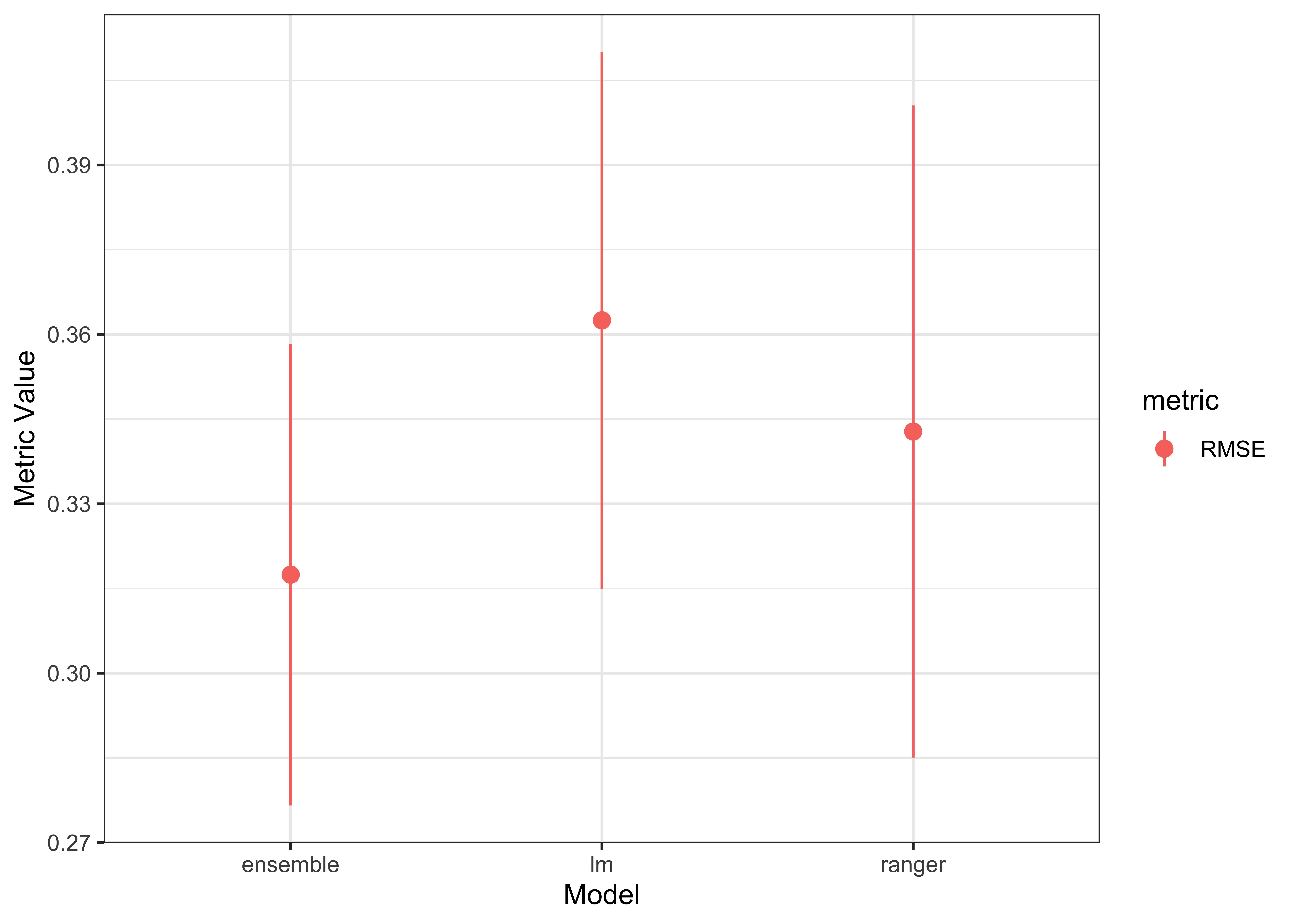
caretEnsemble includes some useful plotting utilities. Use the base plot function to show the error of each model in the stack, as well as the overall error for the stack itself:

plot(glm_stack)

A dot plot comparing the Root Mean Squared Error (RMSE) across three models: ensemble, lm, and ranger. Each model's RMSE is represented by a red dot, with vertical lines showing the standard deviation. The plot indicates that the ensemble model has the lowest average RMSE with a wider range, while the lm model shows a higher average RMSE with the largest spread, and the ranger model falls in between.

Note that while the linear model is generally worse and higher variance than the ranger model, including it in the stack both improves the ensemble and lowers the ensemble’s variance.

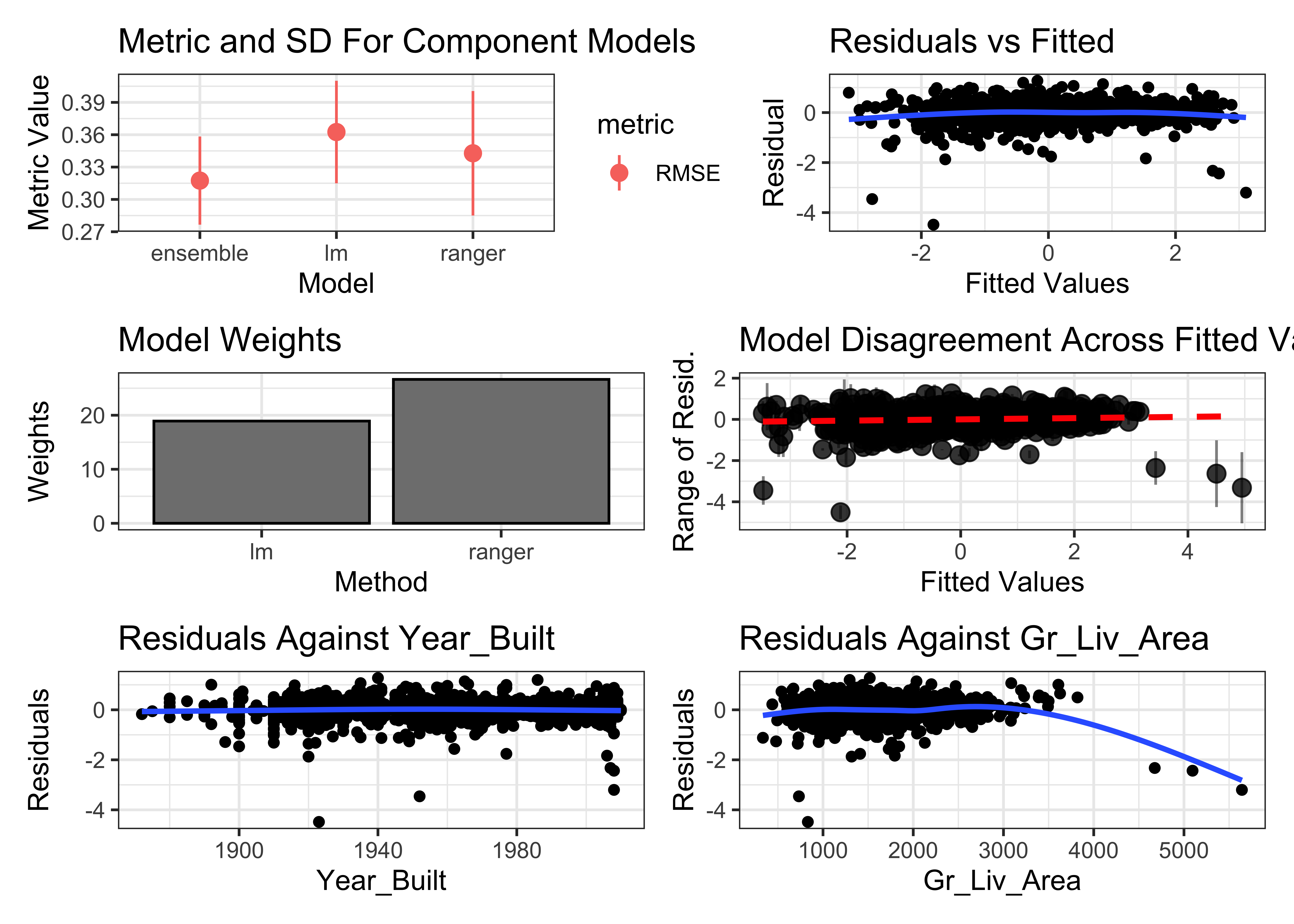
You can also use autoplot from ggplot2 to plot several diagnostics simultaneously:

ggplot2::autoplot(glm_stack, training_data=train_data, xvars=c("Year_Built", "Gr_Liv_Area"))

A multi-panel plot evaluating an ensemble model and its components. The top left panel compares RMSE across the ensemble, lm, and ranger models, showing the ensemble as having the lowest average RMSE. The top middle panel plots residuals against fitted values, indicating potential non-linearity. The top right panel displays model disagreement across fitted values, with a range of residuals. The bottom left panel shows model weights, with lm receiving a higher weight. The bottom middle and bottom right panels display residuals against Year_Built and Gr_Liv_Area, highlighting some patterns and potential model misfits, especially in larger living areas.

The 5 outliers in the training data with high residuals would be a good place to start investigating this model’s performance.

caretEnsemble 4.0

Greedy Ensemble demo

Plots

Further reading

stay in touch