Backtesting Part 4: Random Strategies

Note: This post is NOT financial advice! This is just a fun way to explore some of the capabilities R has for importing and manipulating data.

In part 2, we found that our 200-day high, hold 100 days strategy yielded average annual returns on the S&P 500 index of 7% in a backtest going back to 1950. That’s pretty good, but it’s entirely possible that we got lucky and this was due to chance. One way to test this is to compare our strategy to a strategy that randomly chooses long or short each day. I tested just such a strategy on the S&P 500 index, again going back to 1950. I also adjusted the returns series for splits and dividends, and assumed trade costs were 0.5%. These are the exact same conditions I tested the “high-and-hold” strategy under.

set.seed(1)
nsims <- 1000
library(quantmod)
library(PerformanceAnalytics)

#Load Data
getSymbols('^GSPC',from='1900-01-01')
#> [1] "GSPC"
spyReturns <- dailyReturn(GSPC$GSPC.Adjusted, type = "arithmetic")

#Make 1000 random position vectors
randomPositions <- sample(c(0,1),nsims*length(spyReturns),TRUE)
randomPositions <- matrix(randomPositions,ncol=nsims)

#Determine trades and calculate trade costs
trades <- apply(randomPositions,2,Lag,1) != randomPositions
trades[1,] <- trades[1,]==1
trades <- ifelse(trades,0.001,0) #Assume the commision is 0.5%

#Determine daily returns of random strats
randomStrats <- randomPositions*matrix(rep(spyReturns,nsims),ncol=nsims)
randomStrats <- randomStrats-trades
randomStrats.return <- apply(randomStrats,2,Return.annualized,scale=252)

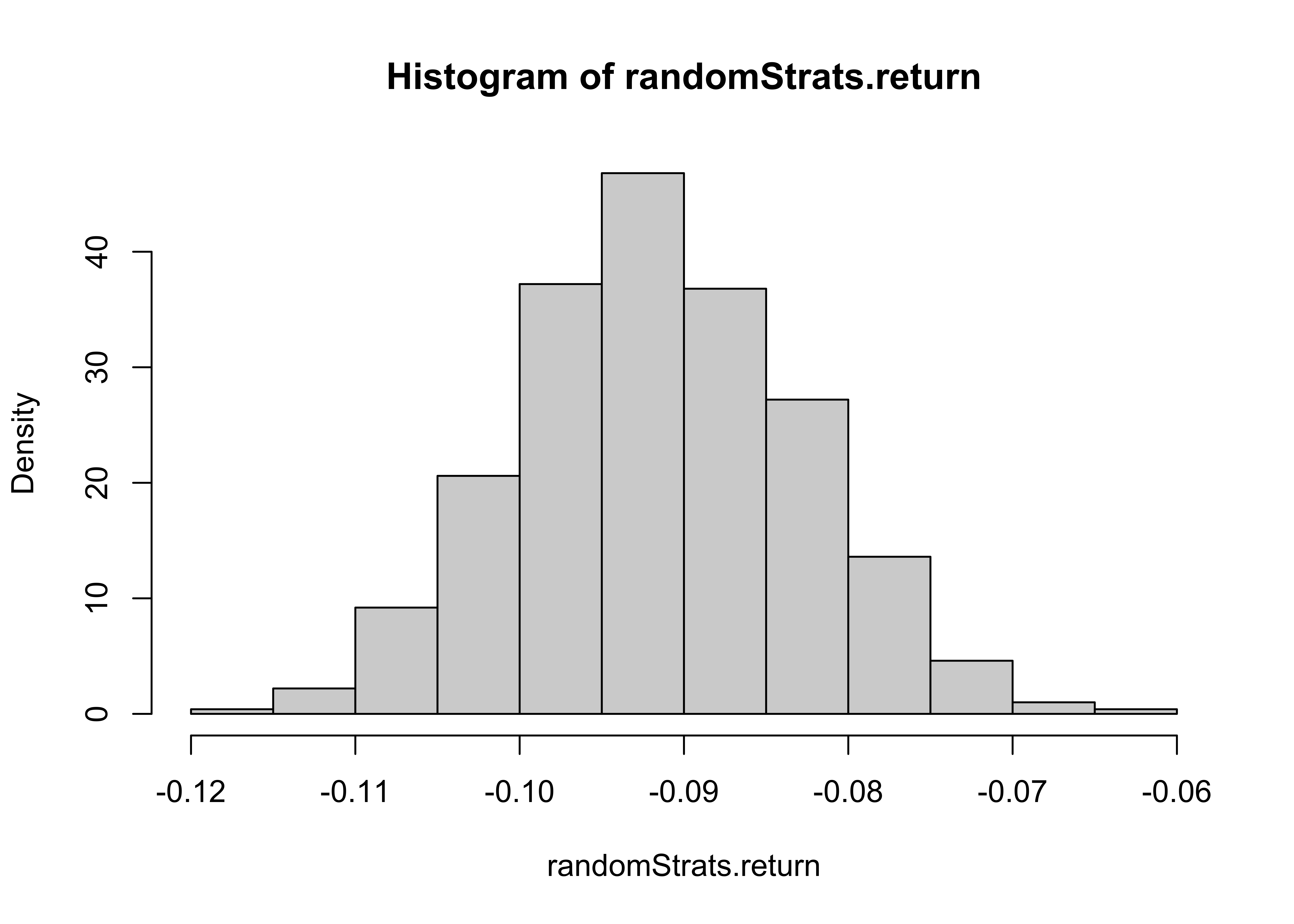
Here is a histogram of average annual returns for these random strategies:

hist(randomStrats.return, freq=FALSE)

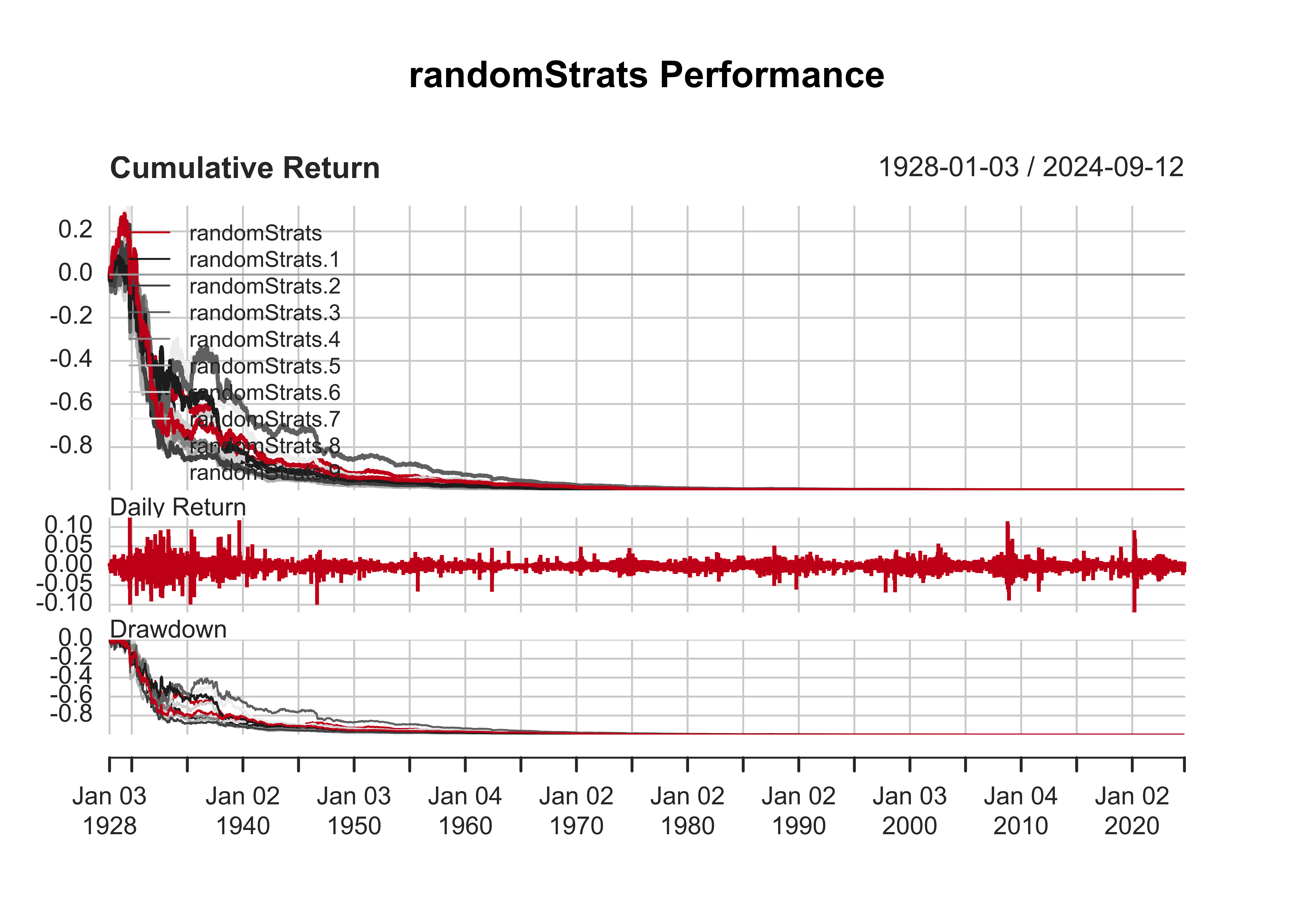
As you can see these strategies perform pretty dismally: the 0.5% trading cost quickly eats up all the available capital.

It would probably be a good idea to model a set dollar amount, and have trades costs a fixed amount, something like $7. It might also be a good idea to make the random strategies auto-correlated, which would probably better reflect actual investor behavior.

charts.PerformanceSummary(na.omit(cbind(spyReturns,randomStrats)[,2:11]),colorset=redfocus)