Backtesting a Simple Stock Trading Strategy
Note: This post is NOT financial advice! This is just a fun way to explore some of the capabilities R has for importing and manipulating data.
UPDATE 9/21/2011: Costas correctly points out that I should lag my strategy vector by one day, as today’s returns are determined the position we chose yesterday. I updated the code, results, and charts to reflect this. Please alert me to any similar errors in the future.
I recently read a post on ETF Prophet that explored an interesting stock trading strategy in Excel. The strategy is simple: Find the high point of the stock over the last 200 days, and count the number of days that have elapsed since that high. If its been more less than 100 days, own the stock. If it’s been more than 100 days, don’t own it. This strategy is very simple, but it yields some impressive results. (Note; however, that this example uses data that has not been adjusted from splits or dividends and could contain other errors. Furthermore, we’re ignoring trading costs and execution delays, both of which affect strategy performance.)
Implementing this strategy in R is simple, and provides numerous advantages over excel, the primary of which is that pulling stock market data into R is easy, and we can test this strategy on a wide range of indexes with relatively little effort.
First of all, we download data for GSPC using quantmod. (GSPC stands for the S&P 500 index). Next, we construct a function to calculate the number of days since the n-day high in a time series, and a function to implement our trading strategy. The latter function takes 2 parameters: the n-day high you wish to use, and the numbers of days past that high you will hold the stock. The example is 200 and 100, but you could easily change this to the 500-day high and see what happens if you hold the stock 300 days past the high before bailing out. Since this function is parameterized, we can easily test many other versions of our strategy. We pad the beginning of our strategy with zeros so it will be the same length as our input data. (If you wish for a more detailed explanation of the daysSinceHigh function, see the discussion on cross-validated).
#http://etfprophet.com/days-since-200-day-highs/
set.seed(42)

require(quantmod)
getSymbols('^GSPC',from='1950-01-01')
#> [1] "GSPC"

daysSinceHigh <- function(x, n){
   apply(embed(x, n), 1, which.max)-1
}

myStrat <- function(x, nHold=100, nHigh=200) {
    position <- ifelse(daysSinceHigh(x, nHigh)<=nHold,1,0)
    c(rep(0,nHigh-1),position)
}

myStock <- Cl(GSPC)
myPosition <- myStrat(myStock,100,200)
bmkReturns <- dailyReturn(myStock, type = "arithmetic")
myReturns <- bmkReturns*Lag(myPosition,1)
myReturns[1] <- 0

names(bmkReturns) <- 'SP500'
names(myReturns) <- 'Me'
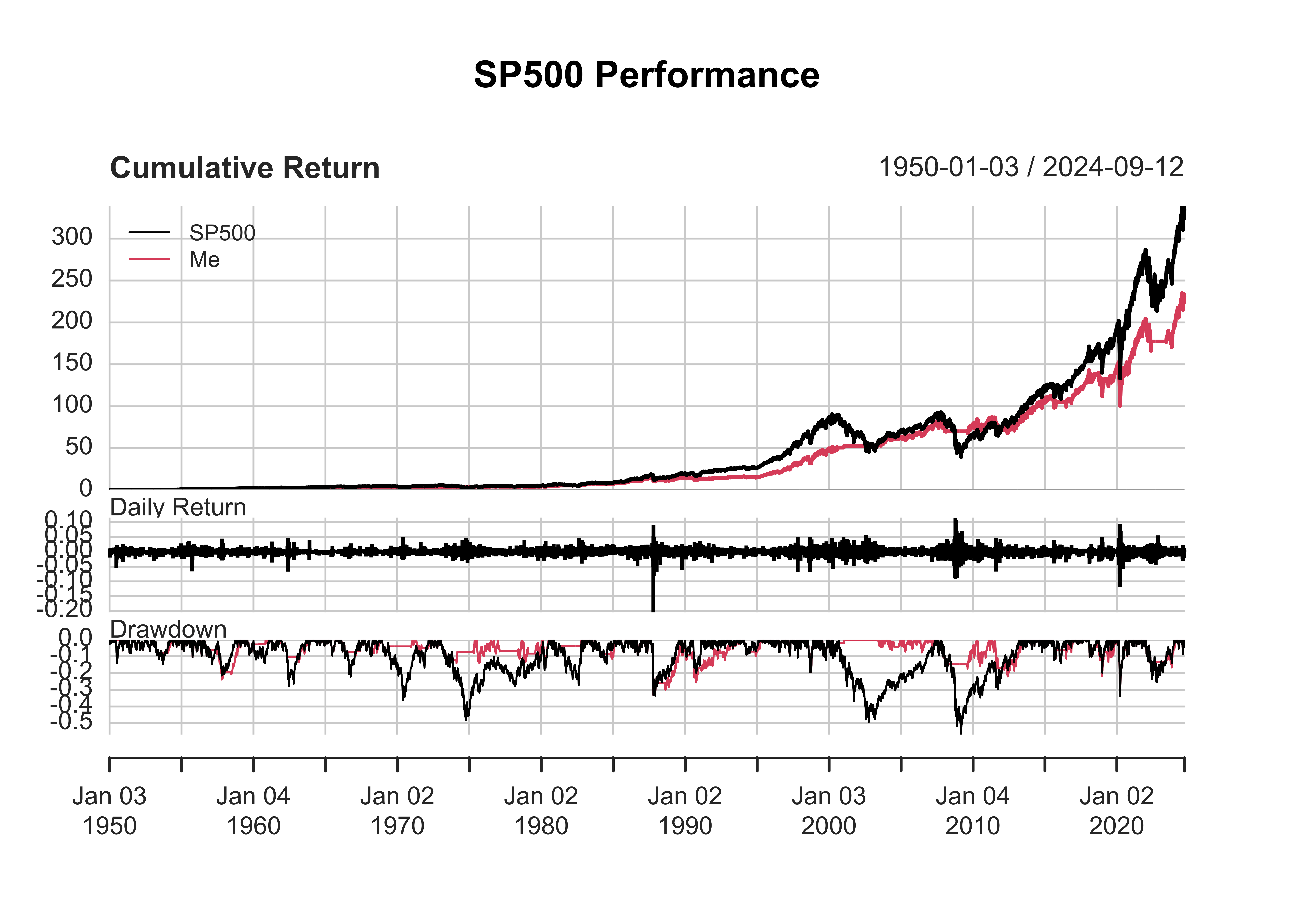
We multiply our position (0,1) vector by the returns from the index to get our strategy’s returns. Now we construct a function to return some statistics about a trading strategy, and compare our strategy to the benchmark. Somewhat arbitrarily, I’ve decided to look at cumulative return, mean annual return, sharpe ratio, winning %, mean annual volatility, max drawdown, and max length drawdown. Other stats would be easy to implement.
Results:
require(PerformanceAnalytics)
charts.PerformanceSummary(cbind(bmkReturns,myReturns))

Performance <- function(x) {

    cumRetx = Return.cumulative(x)
    annRetx = Return.annualized(x, scale=252)
    sharpex = SharpeRatio.annualized(x, scale=252)
    winpctx = length(x[x > 0])/length(x[x != 0])
    annSDx = sd.annualized(x, scale=252)

    DDs <- findDrawdowns(x)
    maxDDx = min(DDs$return)
    maxLx = max(DDs$length)

    Perf = c(cumRetx, annRetx, sharpex, winpctx, annSDx, maxDDx, maxLx)
    names(Perf) = c("Cumulative Return", "Annual Return","Annualized Sharpe Ratio",
        "Win %", "Annualized Volatility", "Maximum Drawdown", "Max Length Drawdown")
    return(round(Perf, 2))
}
cbind(Me=Performance(myReturns),SP500=Performance(bmkReturns))
#>                              Me   SP500
#> Cumulative Return        231.30  333.99
#> Annual Return              0.08    0.08
#> Annualized Sharpe Ratio    0.62    0.51
#> Win %                      0.55    0.53
#> Annualized Volatility      0.12    0.16
#> Maximum Drawdown          -0.34   -0.57
#> Max Length Drawdown     1553.00 1898.00
As you can see, this strategy compares favorably to the default “buy-and-hold” approach.
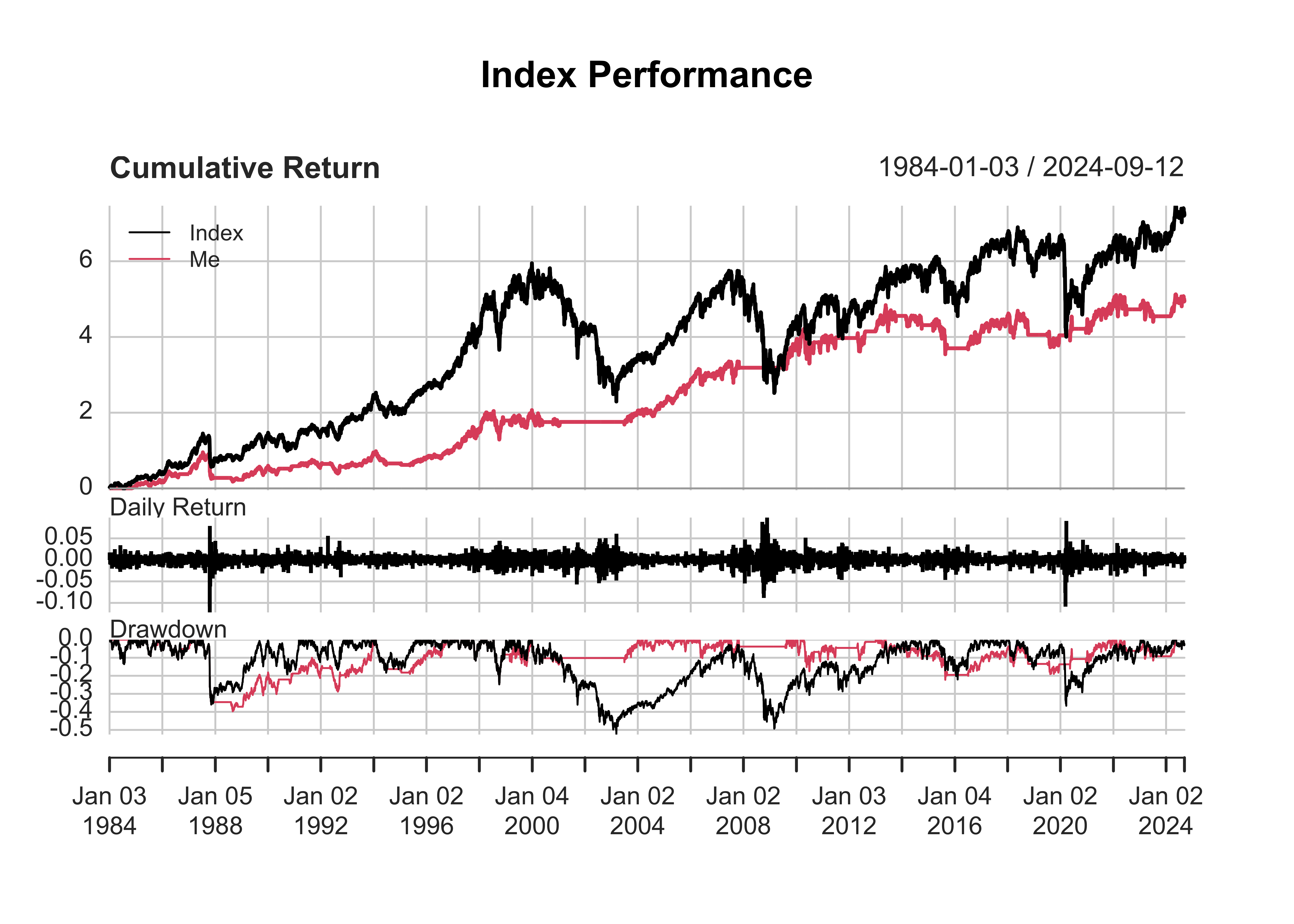
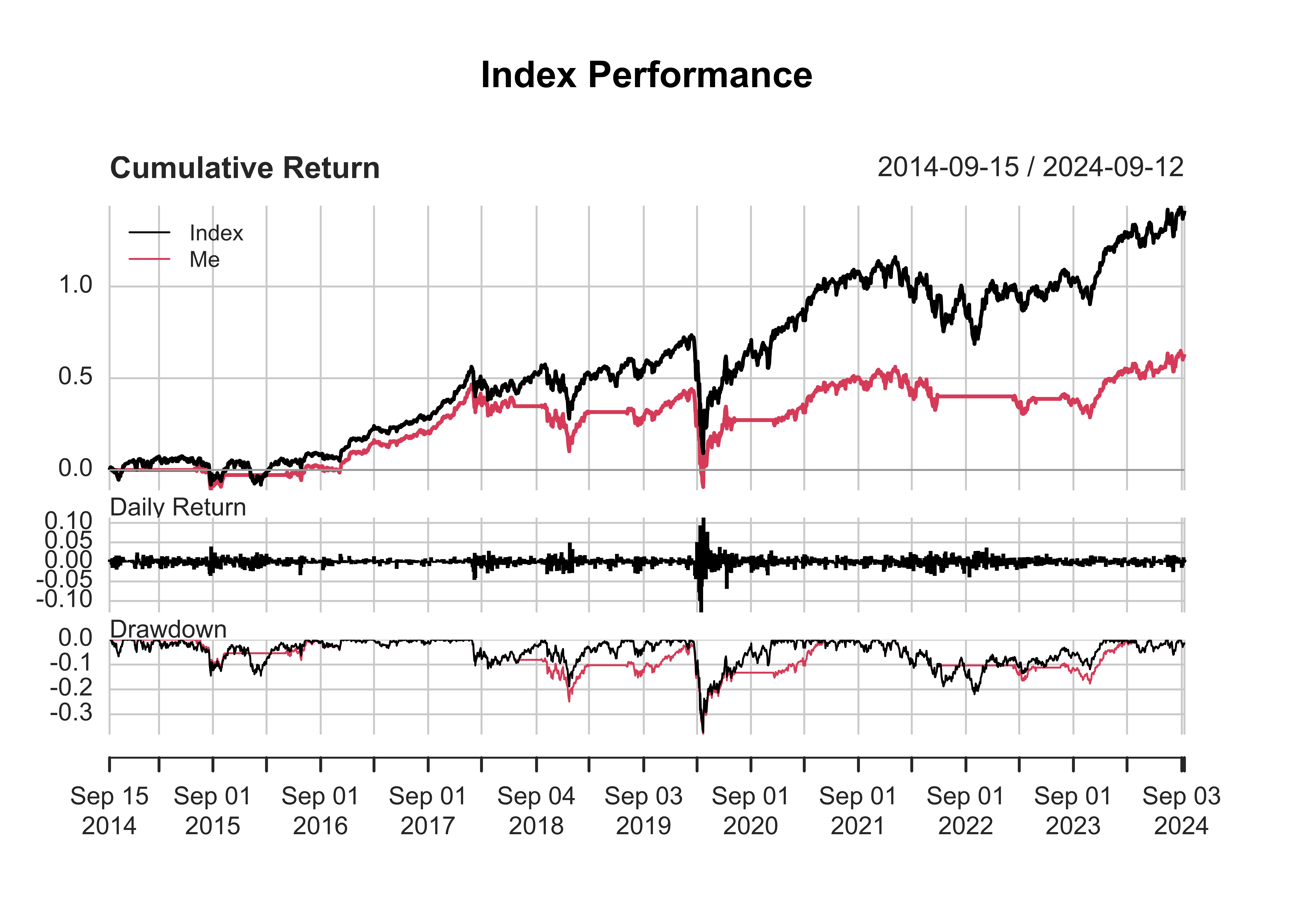
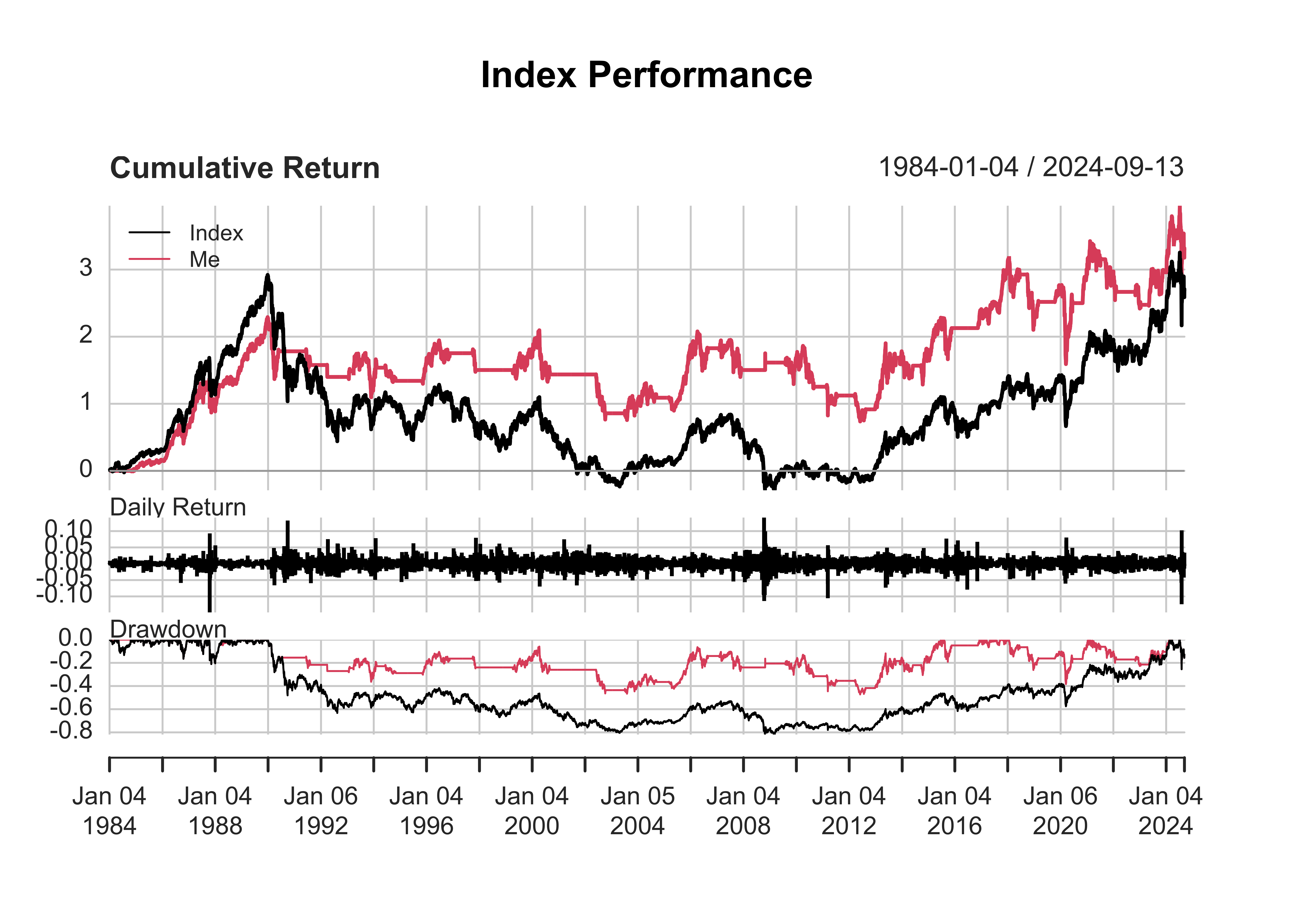
Finally, we test our strategy on 3 other indexes: FTSE which represents Ireland and the UK, the Dow Jones Industrial Index, which goes back to 1896, and the N225, which represents Japan. I’ve functionalized the entire process, so you can test each new strategy with 1 line of code:
testStrategy <- function(myStock, nHold=100, nHigh=200) {
  myStock <- na.omit(myStock)
    myPosition <- myStrat(myStock,nHold,nHigh)
    bmkReturns <- dailyReturn(myStock, type = "arithmetic")
    myReturns <- bmkReturns*Lag(myPosition,1)
    myReturns[1] <- 0
    names(bmkReturns) <- 'Index'
    names(myReturns) <- 'Me'

    charts.PerformanceSummary(cbind(bmkReturns,myReturns))
    cbind(Me=Performance(myReturns),Index=Performance(bmkReturns))

}

getSymbols('^FTSE', from='1984-01-01')
#> [1] "FTSE"
getSymbols('DJIA', src='FRED')
#> [1] "DJIA"
getSymbols('^N225', from='1984-01-01')
#> [1] "N225"
FTSE:
testStrategy(Cl(FTSE),100,200)

#>                              Me   Index
#> Cumulative Return          5.13    7.68
#> Annual Return              0.04    0.05
#> Annualized Sharpe Ratio    0.38    0.31
#> Win %                      0.53    0.53
#> Annualized Volatility      0.12    0.17
#> Maximum Drawdown          -0.40   -0.53
#> Max Length Drawdown     2143.00 3827.00
DJIA:
testStrategy(DJIA,100,200)

#>                             Me  Index
#> Cumulative Return         0.70   1.31
#> Annual Return             0.05   0.09
#> Annualized Sharpe Ratio   0.36   0.50
#> Win %                     0.55   0.54
#> Annualized Volatility     0.15   0.18
#> Maximum Drawdown         -0.38  -0.37
#> Max Length Drawdown     824.00 488.00
N225:
testStrategy(Cl(N225),100,200)

#>                              Me   Index
#> Cumulative Return          3.59    2.74
#> Annual Return              0.04    0.03
#> Annualized Sharpe Ratio    0.25    0.15
#> Win %                      0.53    0.52
#> Annualized Volatility      0.15    0.22
#> Maximum Drawdown          -0.47   -0.82
#> Max Length Drawdown     6622.00 8381.00
The strategy out-performs the other indexes as well. It even performs better than the N225 index, mainly by staying out of it.
Feel free to test this strategy with other parameters, or on other indexes. For homework, think of possible ways that I have fooled myself in this backtest, and post them in the comments. One example of this is that we have’t looked at transaction costs, which might be significant…